# Welcome to Aporia!

Aporia is an ML observability platform that empowers ML teams to monitor and improve their models in production.

Data Science and ML teams rely on Aporia to **visualize** their models in production, as well as **detect and resolve** data drift, model performance degradation, and data integrity issues. 

Aporia offers quick and simple deployment and can monitor billions of predictions with low cloud costs. We understand that use cases vary and each model is unique, that’s why we’ve cemented **customization** at our core, to allow our users to tailor their dashboards, monitors, metrics, and data segments to their needs.

<figure><img src="/files/zd3hIWB1xlVPsPq5EIgo" alt=""><figcaption></figcaption></figure>

## Monitor your models in 3 easy steps&#x20;

<table data-view="cards"><thead><tr><th></th><th></th><th></th><th data-hidden data-card-target data-type="content-ref"></th></tr></thead><tbody><tr><td><strong>Learn</strong></td><td>Learn about data drift, measuring model performance in production across various data segments, and other ML monitoring concepts.</td><td></td><td><a href="/pages/2ZPZvOKuYFChlfBbUgn3">/pages/2ZPZvOKuYFChlfBbUgn3</a></td></tr><tr><td><strong>Connect</strong></td><td>Connect to an existing database where you already store the predictions of your models.</td><td></td><td><a href="/pages/As0DhTP3JOHxTfRlz20Z">/pages/As0DhTP3JOHxTfRlz20Z</a></td></tr><tr><td><strong>Monitor</strong></td><td>Build a dashboard to visualize your model in production and create alerts to notify you when something bad happens.</td><td></td><td><a href="/pages/tg8twL3IZlC8lo3i9EtB">/pages/tg8twL3IZlC8lo3i9EtB</a></td></tr></tbody></table>


# Quickstart

With just a few lines of code, any Machine Learning model can be integrated and monitored in production with Aporia.

![Quickstart](/files/g33AyMj5beT6jc84adTw)

In this guide, we will use Aporia's Python API to create a model in Aporia and log its predictions.

### Install the Aporia SDK

To get started, install the Aporia Python library:

```
pip3 install aporia --upgrade
```

Next, import and initialize the Aporia library:

```python
import aporia
aporia.init(token="<TOKEN>",
            environment="<ENVIRONMENT>",  # e.g prod
            verbose=True,
            raise_errors=True)
```

### Create Model

To create a new model to be monitored in Aporia, you can call the `aporia.create_model(...)` API:

```python
aporia.create_model("<MODEL_ID>", "<MODEL_NAME>")
```

This API will not recreate the model if the model ID already exists. You can also specify color, icon, tags and model owner:

```python
aporia.create_model(
    model_id="fraud-detection",
    model_name="Fraud Detection",
    color=ModelColor.ARCTIC_BLUE,
    icon=ModelIcon.FRAUD_DETECTION,
    tags={
        "framework": "xgboost",
        "coolness_level": 10
    },
    owner="fred@aporia.com", # Integrates with your enterprise auth system ;)
)
```

### Create Model Version

Each model in Aporia contains different **Model Versions**. When you (re)train your model, you should create a new model version in Aporia.

```python
apr_model = aporia.create_model_version(
    model_id="<MODEL_ID>",
    model_version="v1",
    model_type="binary"
    
    features={
        "amount": "numeric",
        "owner": "string",
        "is_new": "boolean",
        "created_at": "datetime",
        "embeddings": {"type": "tensor", "dimensions": [768]},
    },

    predictions={
        "will_buy_insurance": "boolean",
        "proba": "numeric",
    },
)
```

Model version parameter can be any string - you can use the model file's hash, git commit hash, experiment/run ID from MLFlow or anything else.

Model type can be [regression](/v1/model-types/regression), [binary](/v1/model-types/binary), [multiclass](/v1/model-types/multiclass-classification), [multi-label](/v1/model-types/multi-label-classification), or [ranking](/v1/model-types/ranking). Please refer to the relevant documentation on each model type for more info.

#### Field Types

* `numeric` - valid examples: 1, 2.87, 0.53, 300.13
* `boolean` - valid examples: True, False
* `categorical` - a categorical field with integer values
* `string` - a categorical field with string values
* `datetime` - contains either python datetime objects, or an ISO-8601 timestamp string
* `text` - freeform text
* `dict` - dictionaries - at the moment keys are strings and values are numeric
* `tensor` - useful for unstructured data, must specify shape, e.g. `{"type": "tensor", "dimensions": [768]}`

### Log Predictions

Next, we will log some predictions to the newly created model version. These predictions will be kept in an Aporia-managed database.

In production, **we strongly recommend** [**storing your model's predictions in your own database**](/v1/storing-your-predictions/overview) **that you have complete control over**- we've seen many of our customers do this anyway for retraining, auditing, and other purposes.

Aporia can then connect to your data directly and use it for model observability, stripping away the need for data duplication. However, this quickstart assumes you have no database and would simply like to log model inferences:

```python
apr_model.log_prediction(
    id=<PREDICTION_ID>,
    features={
        "amount": 15.3,
        "owner": "Joe",
        "is_new": True,
        "created_at": datetime.now(),
        "embeddings": [...],
    },
    predictions={
        "will_buy_insurance": True,
        "proba": 0.55,
    },
)
```

You must specify an ID for each prediction. This ID can later be used to log the prediction's actual value. If you don't care about this, just pass `str(uuid.uuid4())` as the prediction ID.

Both of these APIs are entirely asynchronous. This was done to avoid blocking your application, which may handle a large number of predictions per second.

You can now access Aporia and see your model, as well as create dashboards and monitors for it!


# Support

Need help? Want something more? Reach out! 📧

### Email Support

Email us and we'll (usually) respond within a few hours, at most 24 hours. 😅

<support@aporia.com>

### Schedule a Call

Schedule a call with one of our team members. We'd be happy to walk you through the platform and help you onboard your first model! 🚀

[Schedule a call](https://www.aporia.com/request-a-demo/)


# Why Monitor ML Models?

You spent *months* working on a sophisticated model, and finally deployed it to production.

8 months later, and the model is still running. Making amazing predictions. Increasing business KPIs by a ton - boss is happy. Satisfied with the results, you move on to this next-gen super cool deep learning computer vision project.

**Sounds like a dream?**

![To Production and Beyond](/files/SOTzJcNPYjcAL3VdI7IH)

***

### The Real Work Begins

Even though we spend a lot of time training and testing our models, *the real work begins when we deploy them to production.* It's one of the most fundamental differences between ML and traditional software engineering.

With traditional software, most of the work is done during the development phase, and once the system is up and running - as long as we've tested it thoroughly - it usually works the way we planned.

With Machine Learning, it *doesn't matter* how well we test our models after training them. **When models run in production, they are exposed to data that's different from what they've been trained on.** Naturally, their performance degrades over time.

### Simple Workflow for ML in Production

Don't panic! Even though models in production do degrade over time, it doesn't mean you'll have to actively take care of each one of them every single minute they're in production.

With two simple principles, you'll be able to move on to that super cool next-gen computer vision project, while knowing your production models are in safe hands:

#### 1. Build a Custom Dashboard

Each one of your models should have a customized production dashboard where you can easily see *the most important metrics* about it. **Put something on your calendar**, and take a look at these dashboards from time to time, to make sure your models are on track!

![Custom Dashboards](/files/PjVtFAqibFw34evSBD9G)

**Bonus points** if you put your dashboard on a big TV screen in the office!

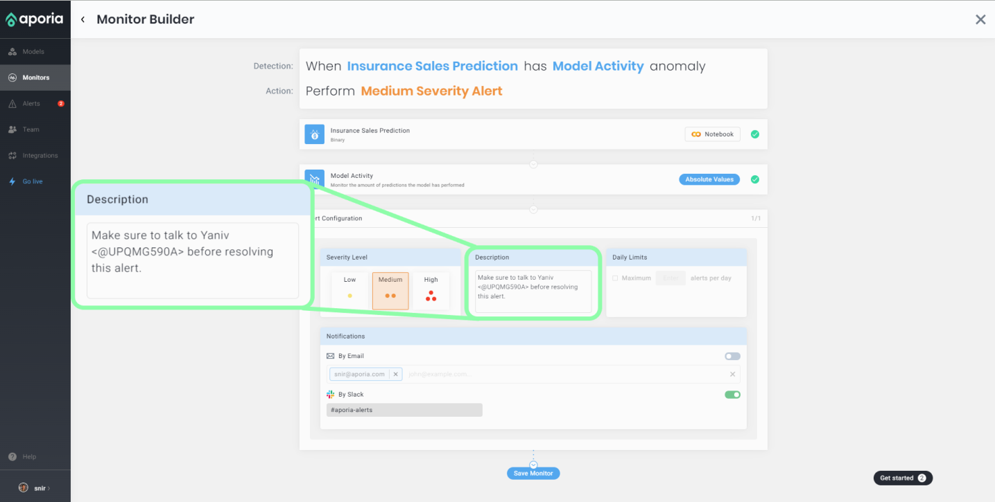
#### 2. Set up important alerts

You should also set up alerts to detect drift, performance degradation, data integrity issues, anomalies in your custom metrics, etc.

To avoid false positives and alert fatigue, make sure to customize the alerts so they only trigger when something important happens.

![Monitor Builder](/files/4BiaYDfDVTLmxgczjOiD)


# Understanding Data Drift

### What is Data Drift?

Data drift occurs when the distribution of *production data* is different from a certain baseline (e.g *training data*).

The model isn't designed to deal with this change in the feature space and so, its predictions may not be reliable. Drift can be caused by changes in the real world or by data pipeline issues - missing data, new values, changes to the schema, etc.

It's important to look at the data that has drifted and follow it back through its pipeline to find out **when** and **where** the drift started.

{% hint style="info" %}
**When should I retrain my model?**

As the data begins to drift, we may not notice significant degradation in our model's performance immediately.

However, this is an excellent opportunity to retrain before the drift has a negative impact on performance.
{% endhint %}

### Measuring Data Drift

To measure how distributions differ from each other, you can use a **statistical distance**. This is a metric that quantifies the distance between two distributions, and it is extremely useful.

There are many different statistical distances for different scenarios.

<figure><img src="/files/SoZ4lULLo5wSdj45Egpr" alt=""><figcaption><p>Is there a data drift here? :)</p></figcaption></figure>

By default, Aporia calculates a metric called **Drift Score**, which is a smart combination of statistical distances such as [Hellinger Distance](https://en.wikipedia.org/wiki/Hellinger_distance) for categorical variables and [Jensen-Shannon Divergence](https://en.wikipedia.org/wiki/Jensen%E2%80%93Shannon_divergence) for numeric variables.

Besides the default drift score, you can customize and add your own statistical distances.

### Intuition to Drift Score

Let's say we have a categorical feature called `pet_type` with 2 possible values:

* 🐶 Dog
* 🐱 Cat

In our training set, the distribution of this feature was **100% 🐶** + **0% 🐱**. This means that when we trained our model, we only had dogs and no cats.

Now, let's evaluate different scenarios in production, and see what would be the drift score:

* If the current distribution is **0% 🐶** + **100% 🐱**, the drift score would be **1.0**.
  * Tons of drift!
* If the current distribution is **50% 🐶** + **50% 🐱**, the drift score would be **0.54**.
* If the current distribution is **60% 🐶** + **40% 🐱**, the drift score would be **0.47**.
* If the current distribution is **100% 🐶** + **0% 🐱**, the drift score would be **0.0**.
  * No drift at all!


# Analyzing Performance

### Your model's success is your success

Hooray! Your model is running in production, making predictions in order to improve your business KPIs.

Unfortunately, when encountering real world pipelines and data our model might not perform as well as it did in our training process.

That's why we would like to analyze our model's performance over-time in order to make sure we catch possible degradation in time.

![It's Performance Review Time](/files/eAUH5Vp1CC1uU6qCs2jh)

### Measuring Model Performance

To measure how well your model performs in production, you can use a variety of **performance metrics**. Each metric teaches us about different aspects of our model's performance.

While some people might care about not missing potential leads (e.g. focus on **recall** score) others might prefer to reduce dead ends to minimum costs (e.g. focus on **precision** score).

In addition, no matter which use case are you trying to solve with your model, you'll probably want to analyze its activity over time and ensure there are no anomalous events or ongoing trends with the model's usage.

{% hint style="info" %}

#### How often should I carry out performance analysis?

As models can vary dramatically in their purpose, usage, or production pipelines, the answer isn't unequivocal.

However, here are some questions you should consider while deciding - What is the frequency of the predictions? How frequently do we get the actuals? Are concept drifts common in this domain?&#x20;
{% endhint %}

### Common Performance metrics

Depending on your use case, you might want to use different performance metrics in order to decide how well our model performs. For example, nDCG is common when you want to understand the quality of your ranking model. AUC-ROC is useful when you want to evaluate you binary classification model.

You can read more about all the different metrics and the use cases which you will find useful in our [metric glossary.](/v1/api-reference/metrics-glossary)<br>

## Actuals / Ground Truth

In some cases, you will have access to the *actual* value of the prediction - the ground truth from real-world data.

For example, if your model predicted that a client will buy insurance, and a few days later the client actually does so, then the actual value of that prediction would be `True`.

In these scenarios, we can compare our predictions to the actual values and then calculate performance metrics like Precision, Recall, MSE, etc. - just like in training.

By connecting Aporia with your actual values, the system will be able to calculate performance metrics in real-time for you.

In this example, you can see the Precision metric across two model versions in production:

<figure><img src="/files/Dmzl1ohA0HRuDyT4mo1T" alt=""><figcaption><p>Timeseries</p></figcaption></figure>


# Tracking Data Segments

Sometimes looking over our entire data doesn't supply us with enough insights to understand what is best to do. We need the ability to break our data into smaller pieces to reach valuable and sharp insights.

This is exactly when data segmentation jumps to our help!

Zooming into a specific data segment can help us understand if our overall performance degradation originates just in that segment or do we have a wide problem. Comparing two different segments can help us decide which one of them is more valuable to invest in our future campaign.

### Tracking Data Segments

There are infinite ways to segment your data. Let us say we want to segment our subjects by their age. What interval between bins should we choose? should that interval be constant or maybe correlating to a real-world segmentation?

Don't be tempted to create them all. Think about what segmentation choice can help you answer real valuable questions that may influence the actions you'll take.

For example, gender is often just raw data and not a feature, but slicing your data by gender can help you surface performance differences or even biases. In such cases, you should consider even monitoring specific issues by segments.


# Models & Versions

### Model

In Aporia, a `model` is any system that can make predictions and can be improved through the use of data.

We use this broad definition in order to support a large number of use cases. Some examples of a model include:

* a simple Pytorch model
* an ensemble of 15 XGBoost models, 37 LightGBM models, and a few deterministic algorithms
* or even an evolutionary algorithm

Aporia models usually serve specific business use cases: Fraud Detection, Credit Risk, Patient Diagnosis, Churn Prediction, LTV, etc.

### Model Version

Each `model` in Aporia can have different `version`. When you (re)train your `model` or update a model's `schema` you should create a new model version in Aporia (via the **Versions page** or **SDK**).

When creating a new model version in Aporia, you'll be able to specify the model version's `schema` - a definition of the inputs and outputs of the model.


# Explainability

**"My model is working perfectly! But why?"**

This is what explainability is all about - the ability to tell *why* your model predicted what it actually predicted. Or, in other words, what is the impact of each feature on the final prediction?

<figure><img src="/files/J6sj3TCpgDob4Z3aPp5p" alt=""><figcaption><p>Explainability in Action</p></figcaption></figure>

### Why Explainability?

There are many reasons why you would need explainability for your models, some examples:

* **Trust:** Models can be viewed as a black box that generates predictions; the ability to explain these predictions increases trust in the model.
* **Debugging:** Being able to explain predictions based on different inputs is a powerful debugging tool for identifying errors.
* **Bias and Fairness:** The ability to see the effect of each feature can aid in identifying unintentional biases that may affect the model's fairness.

For further reading on the subject, check out [our blog about explainability](https://www.aporia.com/blog/explainable-ai/).

### Integrating Explainability in Aporia

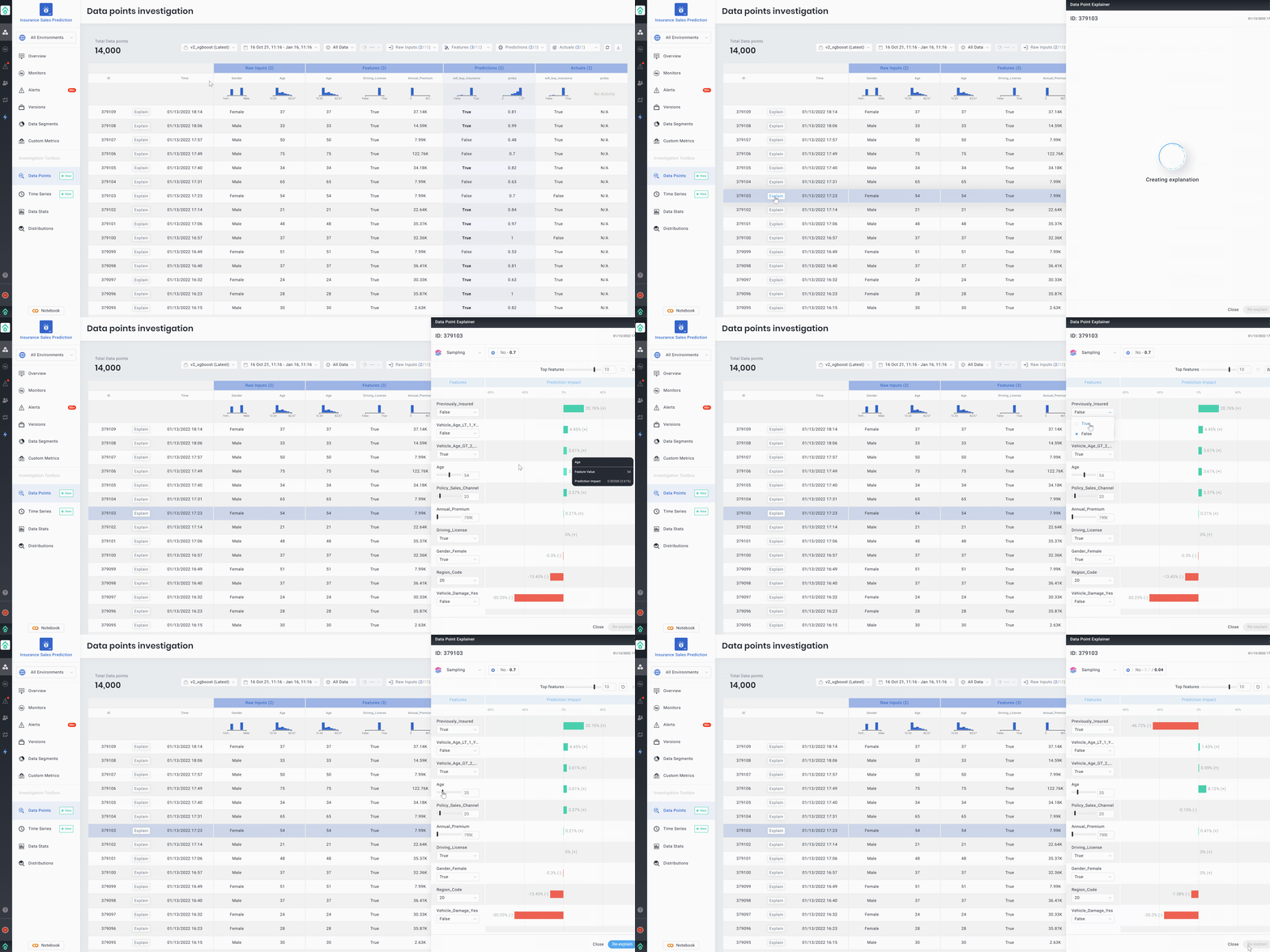
Aporia lets you explain each prediction by visualizing the impact of each feature on the final prediction. This can be done by clicking on the **Explain** button near each prediction in the "Data Points" page of your model.

You can also interactively change any feature value, click **Re-Explain** and see the impact on a theoretical prediction.&#x20;

**Make sure your feature schema in the model version is&#x20;*****ordered***

When creating your model version, you'll need to make sure that the order of the features is identical to your model artifact features.

Instead of passing a normal `dict` as features schema, you'll need to pass `OrderedDict`. For example:

```python
# Build feature schema by order - you can use model.columns for this of course :)
features = OrderedDict()
features["sepal_length"] = "numeric"
features["sepal_width"] = "numeric"
features["petal_length"] = "numeric"
features["petal_width"] = "numeric"

apr_model = aporia.create_model_version(
    model_id="<MODEL_ID>",
    model_version="v1",
    model_type="multiclass",
    features=features,
    predictions={
          "variety": "categorical"
    }
)
```

**Log Training + Serving data**

Training data is required for Explainability. Please check out   [Data Sources - Overview](/v1/data-sources/overview) for more information.

**Upload Model Artifact in ONNX format**

[ONNX](https://onnx.ai/) is an open format for Machine Learning models. Models from all popular ML libraries (XGBoost, Sklearn, Tensorflow, Pytorch, etc.) can be converted to ONNX

To upload your model artifact, you'll need to execute:

```python
apr_model.upload_model_artifact(
    artifact_type="onnx",
    model_artifact=onnx_model.SerializeToString()
)
```

Here are quick snippets and references that may help you with converting your model.

#### XGBoost

```python
import onnxmltools
from onnxmltools.convert.common.data_types import FloatTensorType

initial_types = [('features', FloatTensorType([None, X_train.shape[1]]))]

onnx_model = onnxmltools.convert_xgboost(xgb_model, initial_types=initial_types, target_opset=9)
```

#### LightGBM

```python
import onnxmltools
from onnxmltools.convert.common.data_types import FloatTensorType

initial_types = [('features', FloatTensorType([None, X_train.shape[1]]))]

onnx_model = onnxmltools.convert_lightgbm(lgb_model, initial_types=initial_types, target_opset=9)
```

#### Catboost

```python
import onnxmltools
from onnxmltools.convert.common.data_types import FloatTensorType

initial_types = [('features', FloatTensorType([None, X_train.shape[1]]))]

onnx_model = onnxmltools.covnert_catboost(catboost_model, initial_types=initial_types, target_opset=9)
```

#### Scikit Learn

```python
import onnxmltools
from onnxmltools.convert.common.data_types import FloatTensorType

initial_types = [('features', FloatTensorType([None, X_train.shape[1]]))]

onnx_model = onnxmltools.convert_sklearn(skl_model, initial_types=initial_types, target_opset=9)
```

#### Keras

```python
import onnxmltools

onnx_model = onnxmltools.convert_keras(keras_model, target_opset=9)
```

#### Tensorflow

```python
import onnxmltools

onnx_model = onnxmltools.convert_tensorflow(keras_model, target_opset=9)
```

#### Pytorch

```python
# Please see https://pytorch.org/tutorials/advanced/super_resolution_with_onnxruntime.html
```


# Overview

**Monitoring your Machine Learning models begins with storing their inputs and outputs in production.**&#x20;

Oftentimes, this data is used not just for model monitoring, but also for retraining, auditing, and other purposes; therefore, it is crucial that you have complete control over it.

Aporia monitors your models by connecting directly to *your* data, in *your* format. This section discusses the fundamentals of storing model predictions.

{% hint style="info" %}
If you are not storing your predictions today, you can also [log your predictions directly to Aporia](/v1/storing-your-predictions/logging-to-aporia-directly), although storing your predictions in your own database is highly recommended.
{% endhint %}

### Storage

Depending on your existing enterprise data lake infrastructure, performance requirements, and cloud costs constraints, storing your predictions can be done in a variety of data stores.

Here are some common options:

* [BigQuery](https://cloud.google.com/bigquery)
* [Delta Lake](https://delta.io/) / [Databricks Lakehouse](https://www.databricks.com/)
* [Snowflake](https://www.snowflake.com/)
* [Elasticsearch](https://www.elastic.co/) / [OpenSearch](https://opensearch.org/)
* Parquet files on S3 / GCS / ABS
  * If you choose this option, a metastore such as [Glue Data Catalog](https://docs.aws.amazon.com/glue/latest/dg/catalog-and-crawler.html) is recommended.

### Directory Structure

When storing your predictions, it's highly recommended to adopt a standardized directory structure (or SQL table structure) across all of your organization's models.

With a standardized structure, you'll be able to get all models onboarded to the monitoring system automatically.

Here is a very basic example:

```
s3://myorg-models/
├── my-model/
    ├── v1/
    │   ├── train.parquet
    │   ├── test.parquet
    │   ├── serving.parquet
    │   ├── artifact.onnx
    ├── v2/
    │   ├── train.parquet
    │   ├── test.parquet
    │   └── serving.parquet
    │   └── artifact.onnx
```

{% hint style="info" %}
Even though this section focuses on the storage of *predictions*, you should also consider saving the **training** and **test sets** of your models. They can serve as a monitoring baseline.&#x20;
{% endhint %}

### Data Structure

Recommendations:

* One row per prediction.
* One column per feature, prediction or raw input.
* Use a prefix for column names to identify their group (e.g `features.`, `raw_inputs.`, `predictions.`, `actuals.`, etc.)
* For serving, add ID and prediction timestamp columns.

Example:

```
+-----+----------------------+-------------------+---------------+----------------+-------------------+-------------------------+--------------+----------------------+------------------------+
| id  |      timestamp       | predictions.score | actuals.score | raw_inputs.age | raw_inputs.gender | features.my_embeddings  | features.age | features.gender_male | features.gender_female |
+-----+----------------------+-------------------+---------------+----------------+-------------------+-------------------------+--------------+----------------------+------------------------+
|   1 | 2022-10-19T14:21:08Z |              0.58 |          0.59 |             64 | male              | [0.58, 0.19, 0.38, ...] |           64 |                    1 |                      0 |
|   2 | 2022-10-19T14:21:08Z |              0.64 |          0.66 |             62 | woman             | [0.48, 0.20, 0.42, ...] |           62 |                    0 |                      1 |
| ... | ...                  |               ... |           ... |            ... | ...               | ...                     |          ... |                  ... |                    ... |
+-----+----------------------+-------------------+---------------+----------------+-------------------+-------------------------+--------------+----------------------+------------------------+
```


# Real-time Models (Postgres)

For real-time models with mid-level throughput (e.g models with an HTTP endpoint such as `POST /predict`), you can insert predictions to a database such as [Postgres](https://www.postgresql.org/), [MySQL](https://www.mysql.com/), or even [Elasticsearch](https://www.elastic.co/).

If you are dealing with billions of predictions, this solution might not be sufficient for you.

{% hint style="warning" %}
**Dealing with billions of predictions?**

If you are dealing with billions of predictions, this solution might not be sufficient for you.

Please consider the guide on [real-time models with Kafka](/v1/storing-your-predictions/real-time-models-kafka).&#x20;
{% endhint %}

### Example: FastAPI + SQLAlchemy

If you are serving models with Flask or FastAPI, and don't have an extremely high throughput, you can simply insert predictions to a standard database.

Here, we'll use [SQLAlchemy](https://www.sqlalchemy.org/), which is a Python ORM to replace writing SQL `INSERT` statements directly with something a bit nicer. Please see the [FastAPI + SQLAlchemy tutorial](https://fastapi.tiangolo.com/tutorial/sql-databases/) for more details.

First, we can define the structure of our database table using Pydantic:

```python
class IrisModelPrediction(BaseModel):
    id: str
    timestamp: datetime

    # Features
    sepal_length: float
    sepal_width: float
    petal_length: float
    petal_width: float

    # Predictions
    prediction: int
    confidence: float
```

And here is a sample implementation of `POST /predict` endpoint:

```python
@app.post("/predict")
def predict(request: PredictRequest):
    # Preprocess & predict
    df = pd.DataFrame(columns=['sepal.length', 'sepal.width', 'petal.length', 'petal.width'],
                      data=[[request.sepal.length, request.sepal.width, request.petal.length, request.petal.width]])

    y, confidence = model.predict(df)

    # Insert prediction to DB
    prediction = IrisModelPrediction(
        id=str(uuid.uuid4()),
        timestamp=datetime.now(),
        sepal_length=request.sepal.length,
        sepal_width=request.sepal.width,
        petal_length=request.petal.length,
        petal_width=request.petal.width,
        prediction=y,
        confidence=confidence,
    )

    db.add(prediction)
    db.commit()

    return {"prediction": y_pred}
```


# Real-time Models (Kafka)

For high-throughput, real-time models (e.g models with an HTTP endpoint such as `POST /predict` and billions of predictions per day), you can stream predictions to [Kafka](https://kafka.apache.org/) or other message brokers, and then have a separate process to store them in a persistent storage.

Using a message broker such as Kafka lets you store predictions of real-time models with low latency.

{% hint style="info" %}
**Don't have billions of predictions?**

If you are not dealing with billions of predictions per day, you should consider a simpler solution.

Please see the guide on [real-time models with Postgres](/v1/storing-your-predictions/real-time-models-postgres).
{% endhint %}

### Step 1: Deploy Kafka

You can deploy Kafka in various ways:

* If you are using Kubernetes, you can deploy the [Confluent Helm charts](https://github.com/confluentinc/cp-helm-charts) or the [Strimzi operator](https://strimzi.io/).
* Deploy a managed Kafka service in your cloud provider, e.g [AWS MSK](https://aws.amazon.com/msk/).
* Use a managed service such as [Confluent](https://www.confluent.io/).

### Step 2: Write predictions to Kafka

Writing messages to a Kafka queue is very simple in Python and other languages. Here are examples for Flask and FastAPI, which are commonly used to serve ML models.

#### Flask

With Flask, you can use the [kafka-python](https://kafka-python.readthedocs.io/en/master/) library. Example:

```python
producer = KafkaProducer(bootstrap_servers="kafka-cp-kafka:9092")

@app.route("/predict", methods=["POST"])
def predict():
  ...

  producer.send("my-model", json.dumps({
    "id": str(uuid.uuid4()),
    "model_name": "my-model",
    "model_version": "v1",
    "inputs": {
      "age": 38,
      "previously_insured": True,
    },
    "outputs": {
      "will_buy_insurance": True,
      "confidence": 0.98,
    },
  }).encode("ascii"))    
```

#### FastAPI

With async FastAPI, you can use the [aiokafka](https://aiokafka.readthedocs.io/en/stable/) library. First, initialize a new Kafka producer:

```python
aioproducer = None

@app.on_event("startup")
async def startup_event():
  global aioproducer
  aioproducer = AIOKafkaProducer(bootstrap_servers="my-kafka:9092")

  await aioproducer.start()


@app.on_event("shutdown")
async def shutdown_event():
  await aioproducer.stop()
```

Then, whenever you have a new prediction you can publish it to a Kafka topic:

```python
@app.post("/predict")
async def predict(request: PredictRequest):
  ...

  await aioproducer.send("my-model", json.dumps({
    "id": str(uuid.uuid4()),
    "model_name": "my-model",
    "model_version": "v1",
    "inputs": {
      "age": 38,
      "previously_insured": True,
    },
    "outputs": {
      "will_buy_insurance": True,
      "confidence": 0.98,
    },
  }).encode("ascii"))
```

### Step 3: Stream to a Persistent Storage

Now, you can stream predictions from Kafka to a persistent storage such as S3. There are different ways to achieve this - we'll cover here [Kafka Connect](https://docs.confluent.io/platform/current/connect/index.html) and [Spark Streaming](https://spark.apache.org/docs/latest/streaming-programming-guide.html).

#### Spark Streaming

Spark Streaming is an extension of the core Spark API that allows you to process real-time data from various sources including Kafka. This processed data can be pushed out to file systems and databases.

In this example, we will process messages from the `my-model` topic and store them in a Delta lake table:

```python
# Create stream with Kafka source
df = spark.readStream.format("kafka") \
    .option("kafka.bootstrap.servers", "my-kafka:9092") \
    .option("subscribe", "my-model") \
    .option("startingOffsets", "earliest") \
    .option("failOnDataLoss", "false") \
    .load()


# Parse JSON from Kafka
schema = StructType() \
    .add("sepal_length", FloatType()) \
    .add("sepal_width", FloatType()) \
    .add("petal_length", FloatType()) \
    .add("petal_width", FloatType()) \
    .add("prediction", IntegerType()) \
    .add("confidence", FloatType())

df = df.withColumn("json", F.from_json(F.col("value").cast("string"), schema))
df = df.select(F.col("json.*"))


# Write to Delta Lake
df.writeStream \
    .format("delta") \
    .outputMode("append") \
    .option("mergeSchema", "true") \
    .option("checkpointLocation", f"{S3_BASE_URL}/my-model/serving/_checkpoints/kafka") \
    .start(f"{S3_BASE_URL}/my-model/serving") \
    .awaitTermination()
```

#### Kafka Connect

Kafka Connect makes it easy to quickly define connectors to move data between Kafka and other data systems, such as S3, Elasticsearch, and others.

As a prerequisite to Kafka Connect, you'll need [Schema Registry](https://docs.confluent.io/platform/current/schema-registry/index.html#:~:text=A%20schema%20defines%20the%20structure,that%20scope%20is%20the%20subject%20.), which is a tool to manage schemas for Kafka topics.

Here is an example of a connector to stream messages from the `my-model` topic to Parquet file on S3:

```json
PUT /connectors/my-model-connector/config

{
  "connector.class": "io.confluent.connect.s3.S3SinkConnector",
  "storage.class": "io.confluent.connect.s3.storage.S3Storage",
  "s3.region": "us-east-1",
  "s3.bucket.name": "myorg-models",
  "topics.dir": "my-model/serving",
  "flush.size": "2",
  "rotate.schedule.interval.ms": "20000",
  "auto.register.schemas": "false",
  "tasks.max": "1",
  "s3.part.size": "5242880",
  "timezone": "UTC",
  "parquet.codec": "snappy",
  "topics": "my-model",
  "s3.credentials.provider.class": "com.amazonaws.auth.DefaultAWSCredentialsProviderChain",
  "format.class": "parquet",
  "value.converter": "org.apache.kafka.connect.json.JsonConverter",
  "key.converter": "org.apache.kafka.connect.storage.StringConverter",
  "schema.registry.url": "http://my-schema-registry",
  "value.converter.schema.registry.url": "http://my-schema-registry"
}
```


# Batch Models

If your model runs periodically every X days, we refer to it as a **batch model** (as opposed to a real-time model).

Typically, storing the predictions of batch models is straightforward. The code examples that follow are naive "illustrations" of how to do so.

### Example: Pandas to Parquet on S3

If you use Pandas, you can append any `DataFrame` to a Parquet file on S3 or other cloud storages by using the [fastparquet](https://fastparquet.readthedocs.io/en/latest/) library:

```python
import fastparquet

# Preprocess & predict
X = preprocess(...)
y = model.predict(X_pred)

# Concatenate features, predictions and any other metadata
df = ...

# Store predictions
fastparquet.write(
    filename=f"s3://my-models/{MODEL_ID}/{MODEL_VERSION}/serving.parquet",
    data=df,
    append=True,
)
```

### Example: Pyspark to Delta Lake

This example is especially useful on [Databricks](https://www.databricks.com/), but can you can use it on [Delta Lake](https://delta.io/) + [Spark on K8s operator](https://github.com/GoogleCloudPlatform/spark-on-k8s-operator) for example:

```python
# Predict on SparkML
y = model.transform(X)

# Concatenate features, predictions and any other metadata
df = ...

# Append to a Delta table
df.write.format("delta").mode("append").saveAsTable("my_model_serving")
```


# Kubeflow / KServe

If you are using [Kubeflow](https://www.kubeflow.org/) or [KServe](https://github.com/kserve/kserve) for model serving, you can store the predictions of your models using InferenceDB.

[InferenceDB](https://github.com/aporia-ai/inferencedb) is an open-source cloud native tool that connects to KServe and streams predictions to a data lake, based on Kafka.

{% hint style="warning" %}
**WARNING: InferenceDB is still experimental!**

InferenceDB is an open-source project developed by Aporia. It is still experimental, and not yet ready for production!&#x20;
{% endhint %}

This guide will explain how to deploy a simple scikit-learn model using KServe, and log its inferences to a Parquet file in S3.

### Requirements

* [**KServe**](https://kserve.github.io/website/0.8/)
* [**KNative Eventing**](https://knative.dev/docs/eventing/) - with the [Kafka broker](https://knative.dev/docs/eventing/broker/kafka-broker/)
* [**Kafka**](https://kafka.apache.org/) - with Schema Registry, Kafka Connect, and [Confluent S3 Sink connector](https://docs.confluent.io/kafka-connect-s3-sink/current/overview.html) plugin

To get started as quickly as possible, see the [environment preperation tutorial](https://github.com/aporia-ai/inferencedb/wiki/KServe-Requirements), which shows how to set up a full environment in minutes.

### Step 1: Kafka Broker

First, we will need a Kafka broker to collect all KServe inference requests and responses:

```yaml
apiVersion: eventing.knative.dev/v1
kind: Broker
metadata:
  name: sklearn-iris-broker
  namespace: default
  annotations:
    eventing.knative.dev/broker.class: Kafka
spec:
  config:
    apiVersion: v1
    kind: ConfigMap
    name: inferencedb-kafka-broker-config
    namespace: knative-eventing
---
apiVersion: v1
kind: ConfigMap
metadata:
  name: inferencedb-kafka-broker-config
  namespace: knative-eventing
data:
  # Number of topic partitions
  default.topic.partitions: "8"
  # Replication factor of topic messages.
  default.topic.replication.factor: "1"
  # A comma separated list of bootstrap servers. (It can be in or out the k8s cluster)
  bootstrap.servers: "kafka-cp-kafka.default.svc.cluster.local:9092"
```

### Step 2: InferenceService

Next, we will serve a simple sklearn model using KServe:

```yaml
apiVersion: serving.kserve.io/v1beta1
kind: InferenceService
metadata:
  name: sklearn-iris
spec:
  predictor:
    logger:
      mode: all
      url: http://kafka-broker-ingress.knative-eventing.svc.cluster.local/default/sklearn-iris-broker
    sklearn:
      protocolVersion: v2
      storageUri: gs://seldon-models/sklearn/iris
```

Note the `logger` section - you can read more about it in the [KServe documentation](https://kserve.github.io/website/0.8/modelserving/logger/logger/).

### Step 3: InferenceLogger

Finally, we can log the predictions of our new model using InferenceDB:

```yaml
apiVersion: inferencedb.aporia.com/v1alpha1
kind: InferenceLogger
metadata:
  name: sklearn-iris
  namespace: default
spec:
  # NOTE: The format is knative-broker-<namespace>-<brokerName>
  topic: knative-broker-default-sklearn-iris-broker
  events:
    type: kserve
    config: {}
  destination:
    type: confluent-s3
    config:
      url: s3://aporia-data/inferencedb
      format: parquet

  # Optional - Only if you want to override column names
  schema:
    type: avro
    config:
      columnNames:
        inputs: [sepal_width, petal_width, sepal_length, petal_length]
        outputs: [flower]
```

### Step 4: Send requests

First, we will need to port-forward the Istio service so we can access it from our local machine:

```
kubectl port-forward --namespace istio-system svc/istio-ingressgateway 8080:80
```

Prepare a payload in a file called `iris-input.json`:

```json
{
  "inputs": [
    {
      "name": "input-0",
      "shape": [2, 4],
      "datatype": "FP32",
      "data": [
        [6.8, 2.8, 4.8, 1.4],
        [6.0, 3.4, 4.5, 1.6]
      ]
    }
  ]
}
```

And finally, you can send some inference requests:

```
SERVICE_HOSTNAME=$(kubectl get inferenceservice sklearn-iris -o jsonpath='{.status.url}' | cut -d "/" -f 3)

curl -v \
  -H "Host: ${SERVICE_HOSTNAME}" \
  -H "Content-Type: application/json" \
  -d @./iris-input.json \
  http://localhost:8080/v2/models/sklearn-iris/infer
```

### Step 5: Success!

If everything was configured correctly, these predictions should have been logged to a Parquet file in S3.

```python
import pandas as pd

df = pd.read_parquet("s3://aporia-data/inferencedb/default-sklearn-iris/")
print(df) 
```

[See the full example here.](https://github.com/aporia-ai/inferencedb/tree/main/examples/kserve/kafka-broker)


# Logging to Aporia directly

This section will teach you how to integrate Aporia using [Python SDK](https://aporia-sdk-ref.netlify.app/), but you can also use our [REST API](/v1/api-reference/rest-api) or the integrate to your own DB.

## Get Started

To get started, install the Aporia SDK:

```bash
pip3 install aporia --upgrade
```

And then initialize it in your code:

```python
import aporia
aporia.init(token="<TOKEN>",
            environment="<ENVIRONMENT>", # e.g "production"
            verbose=True,
            raise_errors=True)
```

### Create Model

To create a new model to be monitored in Aporia, you can call the `aporia.create_model(...)` API:

```python
aporia.create_model("<MODEL_ID>", "<MODEL_NAME>")
```

This API would not recreate the model if the model ID already exists. You can also specify color, icon, tags, and model owner:

```python
aporia.create_model(
    model_id="fraud-detection",
    model_name="Fraud Detection",
    color=ModelColor.ARCTIC_BLUE,
    icon=ModelIcon.FRAUD_DETECTION,
    tags={
        "framework": "xgboost",
        "coolness_level": 10
    },
    owner="fred@aporia.com", # Integrates with your enterprise auth system ;)
)
```

### Create Model Version

Each model in Aporia contains different **Model Versions**. When you (re)train your model, you should create a new model version in Aporia.

**Manual**

```python
apr_model = aporia.create_model_version(
  model_id="<MODEL_ID>",
  model_version="v1",
  model_type="binary",
  features={
    "amount": "numeric",
    "owner": "string",
    "is_new": "boolean",
    "created_at": "datetime",
  },
  predictions={
    "will_buy_insurance": "boolean",
    "proba": "numeric",
  },
  # Optional
  feature_importance={
    "amount": 80,
    "owner": 10,
    "is_new": 70,
    "created_at": 20,
  }
)
```

**Inferring from Pandas DataFrame**

```python
# Example DataFrames, each one with one row
features_df = pd.DataFrame([[12.3, "John", True, pd.Timestamp.now()]], 
  columns=["amount", "owner", "is_new", "created_at"])

predictions_df = pd.DataFrame([[True, 0.7]], 
  columns=["will_buy_insurance", "proba"])


# Create a model version by inferring schemas from pandas DataFrames
apr_model = aporia.create_model_version(
    model_id="<MODEL_ID>",
    model_version="v1",
    model_type="binary",

    features=aporia.pandas.infer_schema_from_dataframe(features_df),
    predictions=aporia.pandas.infer_schema_from_dataframe(predictions_df),
      
    # Optional
    feature_importance={
      "amount": 80,
      "owner": 10,
      "is_new": 70,
      "created_at": 20,
    }
)
```

Model version parameter can be any string - you can use the model file's hash, git commit hash, experiment/run ID from MLFlow or anything else.

Model type can be [regression](/v1/model-types/regression), [binary](/v1/model-types/binary), [multiclass](/v1/model-types/multiclass-classification), [multi-label](/v1/model-types/multi-label-classification), or [ranking](/v1/model-types/ranking). Please refer to the relevant documentation on each model type for more info.

#### Field Types

* `numeric` - valid examples: 1, 2.87, 0.53, 300.13
* `boolean` - valid examples: True, False
* `categorical` - a categorical field with integer values
* `string` - a categorical field with string values
* `datetime` - contains either python datetime objects, or an ISO-8601 timestamp string
* `text` - freeform text
* `dict` - dictionaries - at the moment keys are strings and values are numeric
* `tensor` - useful for unstructured data, must specify shape, e.g. `{"type": "tensor", "dimensions": [768]}`
* `vector` - useful for arrays that can be different in sizes

#### Get a reference to an existing version

If you already created a version, for example during your training, and you want to use it again, you can receive a reference to the version.

```python
apr_model = aporia.Model("<MODEL_ID>", "v1")
```

## Logging Training / Test Sets

To log the training or test sets of your model, you can use the `apr_model.log_training_set` or `apr_model.log_test_set` functions, respectively.

For example, if we have the following training set:

```python
import pandas as pd

training_features = pd.DataFrame({
  "Age": [31, 20, 53],
  "Annual_Premium": [11234, 534534, 859403],
  "Previously_Insured": [False, True, True],
  "Vehicle_Age_LT_1_Year": [False, True, False],
  "Vehicle_Age_GT_2_Years": [True, False, True],
  "Vehicle_Damage_Yes": [True, False, False],
})

training_predictions = pd.DataFrame({
  "will_buy_insurance": [True, True, False],
})

training_labels = pd.DataFrame({
  "will_buy_insurance": [True, False, True],
})
```

Then you can run:

```
apr_model.log_training_set(
  features=training_features,
  predictions=training_predictions,
  labels=training_labels,
)
```

And similarly, you can use the `apr_model.log_test_set` to log your test set.

In both functions, you can pass `raw_inputs` to log the raw inputs of your training / test sets.

## Logging Serving Data

### Log Predictions

Use the `apr_model.log_prediction` API to log a new prediction.

```python
apr_model.log_prediction(
  id=<PREDICTION_ID>,
  features={
    "amount": 15.3,
    "owner": "Joe",
    "is_new": True,
    "created_at": datetime.now(),
  },
  predictions={
    "will_buy_insurance": True,
    "proba": 0.55,
  },
)
```

Note that for each prediction you must specify an ID. This ID can later be used to log the *actual* value of the prediction. If you don't care about actuals, you can simply pass `str(uuid.uuid4())` as prediction ID.

After logging your first prediction you'll be able to get into your model page on the dashboard.

To log multiple predictions in one call, check out [Batching](#batching).

### Raw Inputs

Raw inputs are the inputs of the model *before* preprocessing, and they're used to construct the features. Logging them is optional but can help you detect issues in your data pipeline.

**Example: Log raw inputs separately**

```python
apr_model.log_raw_inputs(
  id="a4dfcd4c-356c-4eed-8b93-b129b64fd55c",
  raw_inputs={
    "Age": 27,
    "Vehicle_Damage": "Yes",
    "Annual_Premium": 12345,
    "Vehicle_Age": ">2 years"
  },
)
```

**Example: Log raw inputs in `log_prediction`**

```python
apr_model.log_prediction(
  id="a4dfcd4c-356c-4eed-8b93-b129b64fd55c",
  features={
    "Age": 27,
    "Vehicle_Damage_Yes": True,
    "Annual_Premium": 12345,
    "Vehicle_Age_LT_1_Year": False,
    "Vehicle_Age_GT_2_Years": True,
  },
  predictions={
    "will_buy_insurance": True,
  },
  raw_inputs={
    "Age": 27,
    "Vehicle_Damage": "Yes",
    "Annual_Premium": 12345,
    "Vehicle_Age": ">2 years"
  },
)
```

### Actuals

In some cases, you will have access to the [actual value](https://github.com/aporia-ai/docs2/blob/main/core-concepts/actuals-ground-truth/README.md) of the prediction, based on real-world data.

For example, if your model predicted that a client will buy insurance, and a day later the client actually makes a purchase, then the actual value of that prediction is `True`

**Example: Log actuals separately**

```python
apr_model.log_actuals(
  id="a4dfcd4c-356c-4eed-8b93-b129b64fd55c",
  actuals={
    "will_buy_insurance": True,
  },
)
```

**Example: Log actuals in `log_prediction`**

```python
apr_model.log_prediction(
  id="a4dfcd4c-356c-4eed-8b93-b129b64fd55c",
  features={
    "Age": 27,
    "Vehicle_Damage_Yes": True,
    "Annual_Premium": 12345,
    "Vehicle_Age_LT_1_Year": False,
    "Vehicle_Age_GT_2_Years": True,
  },
  predictions={
    "will_buy_insurance": True,
  },
  actuals={
    "will_buy_insurance": True,
  },
)
```

### Batching

All of the function above log a single prediction. If you wish to log multiple predictions in one large batch, you can use the `log_batch_*` functions.

Each of these functions receive a list of dictionaries, such that each dict contains the parameters of the singular version of the function.

**Example: Logging batch predictions**

```python
apr_model.log_batch_prediction(
  [
    {
      "id":"a4dfcd4c-356c-4eed-8b93-b129b64fd55c",
      "features": {
        "Age": 27,
        "Vehicle_Damage_Yes": True,
        "Annual_Premium": 12345,
        "Vehicle_Age_LT_1_Year": False,
        "Vehicle_Age_GT_2_Years": True,
      },
      "predictions": {
        "will_buy_insurance": True,
      },
    },
    {
      "id":"f2d1dccb-1aef-4955-a274-69e1acb8772f",
      "features": {
        "Age": 54,
        "Vehicle_Damage_Yes": False,
        "Annual_Premium": 54324,
        "Vehicle_Age_LT_1_Year": True,
        "Vehicle_Age_GT_2_Years": False,
      },
      "predictions": {
        "will_buy_insurance": False,
      },
    },
  ]
)
```

**Example: Logging batch actuals**

```python
apr_model.log_batch_actuals(
  [
    {
      "id":"a4dfcd4c-356c-4eed-8b93-b129b64fd55c",
      "actuals": {
        "will_buy_insurance": True,
      },
    },
    {
      "id":"f2d1dccb-1aef-4955-a274-69e1acb8772f",
      "actuals": {
        "will_buy_insurance": False,
      },
    },
  ]
)
```

**Example: Logging batch raw inputs**

```python
apr_model.log_batch_raw_inputs(
  [
    {
      "id":"a4dfcd4c-356c-4eed-8b93-b129b64fd55c",
      "raw_inputs": {
        "Age": 27,
        "Vehicle_Damage": "Yes",
        "Annual_Premium": 12345,
        "Vehicle_Age": ">2 years"
      },
    },
    {
      "id":"f2d1dccb-1aef-4955-a274-69e1acb8772f",
      "raw_inputs": {
        "Age": 54,
        "Vehicle_Damage": "No",
        "Annual_Premium": 54324,
        "Vehicle_Age": "<1 Year"
      },
    },
  ]
)
```

### Logging Pandas DataFrame / Series

If the data you wish to log is stored in a Pandas Series or DataFrame (with a single row), you can use the `aporia.pandas` utility API:

```python
from aporia.pandas.pandas_utils import pandas_to_dict

apr_model.log_prediction(
  id="a4dfcd4c-356c-4eed-8b93-b129b64fd55c",
  features=pandas_to_dict(features_dataframe),
  predictions={
    "will_buy_insurance": True,
  },
)
```

### Asynchronous logging

All of the logging functions described above log the data asynchronously to avoid blocking your program. If you wish to wait for the data to be sent, you can use the `flush` method:

```python
apr_model.flush()
```

### Troubleshooting

By default, the Aporia SDK is very silent: **it doesn't raise exceptions and doesn't write debug logs.** This was done because we never want to interrupt your application!

However, when first playing with the Aporia SDK, we highly recommend using the verbose argument, e.g:

```python
aporia.init(..., verbose=True)
```

This will print errors in a convenient way to make integration easier to debug. You can also pass `throw_errors=True`, which will make sure you aren't missing any errors.

If you have any further issues, please [contact us](mailto:support@aporia.com).

**Important:** Make sure to remove `throw_errors=True` before uploading to staging / production!

{% hint style="danger" %}
**Prediction isn't sent?**

If your application exits immediately after logging a prediction, the prediction might get discarded.

The reason for this is that predictions are added to a queue and are sent asynchronously.

In order to fix this, use the following API:

`apr_model.flush()`
{% endhint %}

## Pyspark

To log a Pyspark DataFrames directly, you can use the:

* `apr_model.log_batch_pyspark_prediction` for serving data
* `apr_model.log_pyspark_training_set` for training set
* `apr_model.log_pyspark_test_set` for test set

The API of these functions is similar to the `connect_serving` API (see [Data Sources - Overview](/v1/data-sources/overview)).

Example:

```python
import aporia
aporia.init(host="<HOST>", 
            token="<TOKEN>", 
            environment="<ENVIRONMENT>", 
            verbose=True,
            raise_errors=True)


# Create a new model + model version in Aporia
model_id = aporia.create_model("my-model", "My Model")
apr_model = aporia.create_model_version(
    model_id=model_id,
    model_version="v1",
    model_type="binary",
    features={
      "f1": "numeric",
      "f2": "numeric",
      "f3": "numeric",
    },
    predictions={
      "score": "boolean",
    },
)

# Log training set
# We'll assume that there is a column in the dataframe for each feature / prediction
df_train = spark.sql("SELECT * FROM ...")
apr_model.log_pyspark_training_set(df)


# Load & log production data to Aporia
# We'll assume that there is a column in the dataframe for each feature / prediction
df = spark.sql("SELECT * FROM <>")
apr_model.log_batch_pyspark_prediction(
    data=df,

    # Names of the "ID" and "occurred_at" columns
    id_column="id",
    timestamp_column="occurred_at",

    # Map an prediction (from the schema) to a label
    labels={
        "<PREDICTION_NAME>": "<COLUMN_NAME>",
    },
)
```


# Regression

Regression models predict a `numeric` value. In Aporia, these models are represented with the `regression` model type.

Examples of regression problems:

* What will the temperature be in Seattle tomorrow?
* For product X, how many units will sell?
* How many days until this customer stops using the application?
* What price will this house sell for?

### Integration

Regression predictions are usually represented in a database with a `numeric` column. For example:

<table><thead><tr><th width="93">id</th><th width="116">feature1 (numeric)</th><th width="121">feature2 (boolean)</th><th width="215">predicted_temperature (numeric)</th><th width="190">actual_temperature (numeric)</th><th width="193">timestamp (datetime)</th></tr></thead><tbody><tr><td>1</td><td>13.5</td><td>True</td><td>22.83</td><td>24.12</td><td>2017-01-01 12:00:00</td></tr><tr><td>2</td><td>123</td><td>False</td><td>26.04</td><td>25.99</td><td>2017-01-01 12:01:00</td></tr><tr><td>3</td><td>42</td><td>True</td><td>29.01</td><td>11.12</td><td>2017-01-01 12:02:00</td></tr></tbody></table>

To monitor this model, we will create a new model version with a schema that includes a `numeric` prediction:

```python
apr_model = aporia.create_model_version(
  model_id="<MODEL_ID>", # You will need to create a model with this MODEL_ID in advance
  model_version="v1",
  model_type="regression"
  features={
     ...
  },
  predictions={
    "predicted_temperature": "numeric",
  },
)
```

To connect this model to Aporia from your data source, call the `connect_serving(...)` API:&#x20;

```python
apr_model.connect_serving(
  data_source=my_data_source,

  id_column="id",
  timestamp_column="timestamp",

  # Map the actual_temperature column as the label for the 
  # predicted_temperature. 
  labels={
    # Prediction name -> Column name
    "predicted_temperature": "actual_prediction"
  }
)
```

Check out the [data sources section](/v1/data-sources/overview) for more information about how to connect all other available data sources.

{% hint style="info" %}
**Don't want to connect to a database?**

Don't worry - you can [log your predictions directly to Aporia.](/v1/storing-your-predictions/logging-to-aporia-directly)
{% endhint %}


# Binary Classification

Binary classification models predict a binary outcome (one of two possible classes). In Aporia, these models are represented by the binary model type.

Examples of binary classification problems:

* Will the customer `buy` this product or `not_buy` this product?
* Is this email `spam` or `not_spam`?
* Is this review written by a `customer` or a `robot`?

Frequently, binary models output not only a yes/no answer, but also a *probability*.

### Example: Boolean Decision without Probability

If you have a model with a yes/no decision but without a probability value, then your database may look like the following:

<table><thead><tr><th width="76">id</th><th width="132">feature1 (numeric)</th><th width="141">feature2 (boolean)</th><th width="122">decision (boolean)</th><th>label (boolean)</th><th width="191">timestamp (datetime)</th></tr></thead><tbody><tr><td>1</td><td>13.5</td><td>True</td><td>True</td><td>True</td><td>2014-10-19 10:23:54</td></tr><tr><td>2</td><td>-8</td><td>False</td><td>False</td><td>True</td><td>2014-10-19 10:24:24</td></tr></tbody></table>

To monitor this model, we will create a new model version with a schema that include a `boolean` prediction:

```python
apr_model = aporia.create_model_version(
  model_id="<MODEL_ID>",
  model_version="v1",
  model_type="binary"
  features={
     ...
  },
  predictions={
    "decision": "boolean",
  },
)
```

To connect this model to Aporia from your data source, call the `connect_serving(...)` API:&#x20;

```python
apr_model.connect_serving(
  data_source=my_data_source,

  id_column="id",
  timestamp_column="timestamp",

  # Map the "label" column as the label for the "decision" prediction. 
  labels={
    # Prediction name -> Column name
    "decision": "label"
  }
)
```

Check out the [Data Sources](/v1/data-sources/overview) section for further reading on the available data sources and how to connect to each one of them.

### Example: Boolean Decision with Probability

If you have a model with a yes/no decision *and* a probability / confidence value for it, then your database may look like the following:

<table><thead><tr><th width="82">id</th><th width="116">feature1 (numeric)</th><th width="112">feature2 (boolean)</th><th width="112">proba (numeric)</th><th width="138">decision (boolean)</th><th width="122">label (boolean)</th><th width="196">timestamp (datetime)</th></tr></thead><tbody><tr><td>1</td><td>13.5</td><td>True</td><td>0.8</td><td>True</td><td>True</td><td>2014-10-19 10:23:54</td></tr><tr><td>2</td><td>-8</td><td>False</td><td>0.5</td><td>False</td><td>True</td><td>2014-10-19 10:24:24</td></tr></tbody></table>

To monitor this model, it's recommended to create a new model version with a schema that includes the final decision as `boolean` field, and the probability as a `numeric` field:

```python
apr_model = aporia.create_model_version(
  model_id="<MODEL_ID>",
  model_version="v1",
  model_type="binary"
  features={
     ...
  },
  predictions={
    "decision": "boolean",
    "proba": "numeric",
  },
)
```

To connect the model to Aporia from a data source, call the `connect_serving(...)` API:&#x20;

```python
apr_model.connect_serving(
  data_source=my_data_source,
    
  id_column="id",
  timestamp_column="timestamp",

  # Map the "label" column as the label for "decision" and "proba". 
  labels={
    # Prediction name -> Column name representing 
    "decision": "label",
    "proba": "label",
  }
)
```

Check out the [Data Sources](/v1/data-sources/overview) section for further reading on the available data sources and how to connect to each one of them.

### Example: Probability Only

In cases when there is no threshold for your boolean prediction, and the final business result is actually a probability, you may simply omit the `decision` field from the examples in the previous section and only include the `proba` field for your prediction.&#x20;

{% hint style="info" %}
**Don't want to connect to a database?**

Don't worry - you can [log your predictions directly to Aporia.](/v1/storing-your-predictions/logging-to-aporia-directly)
{% endhint %}


# Multiclass Classification

Multiclass classification models predict one of more than two outcomes. In Aporia, these models are represented with the `multiclass` model type.

Examples of multiclass classification problems:

* Is this product a book, movie, or clothing?
* Is this movie a romantic comedy, documentary, or thriller?
* Which category of products is most interesting to this customer?

Frequently, multiclass models output a confidence value or a score for each class.

### Integration

To monitor a multiclass model, create a new model version with a `string` field representing the predicted class, and optionally a `dict` field with the probabilities for all classes:

```python
apr_model = aporia.create_model_version(
  model_id="<MODEL_ID>",
  model_version="v1",
  model_type="multiclass"
  features={
     ...
  },
  predictions={
    "product_type": "string",
    "proba": "dict"
  },
)
```

Next, connect to a data source or manually log predictions like so:

```python
apr_model.log_prediction(
  id="<PREDICTION_ID>",
  features={
    ...
  },
  predictions={
    "product_type": "book",
    "proba": {
        "book": 0.8,
        "movie": 0.1,
        "clothing": 0.1
    }
  },
)
```

To log actuals for this prediction:

```python
apr_model.log_actuals(
  id="<PREDICTION_ID>",
  actuals={
    "product_type": "book",
    "proba": {
        "book": 1.0,
        "movie": 0.0,
        "clothing": 0.0,
    },
  },
)
```

If you don't need to monitor probabilities, you may omit the `proba` field.


# Multi-Label Classification

Multi-label classification models predict multiple outcomes. In Aporia, these models are represented with the `multi-label` model type.

Examples of multi-label classification problems:

* Is this song sad, happy, funny, rock, jazz, or all simultaneously?
* Does this movie belong to one or more of the 'romantic', 'comedy', 'documentary', 'thriller' categories, or all simultaneously?

### Integration

To monitor a multi-label model, create a new model version with a `dict` field where keys are different labels and values are the probabilities for each label:

```python
apr_model = aporia.create_model_version(
  model_id="<MODEL_ID>",
  model_version="v1",
  model_type="multi-label"
  features={
     ...
  },
  predictions={
    "genres": "dict"
  },
)
```

Next, connect to a data source or manually log predictions like so:

```python
apr_model.log_prediction(
  id="<PREDICTION_ID>",
  features={
    ...
  },
  predictions={
    "genres": {
        "action": 0.8,
        "horror": 0.7,
        "thriller": 0.9,
        "drama": 0.2,
        ...
    }
  },
)
```

If you don't have probabilities for each label, you can log zeros and ones instead. To log actuals for this prediction:

```python
apr_model.log_actuals(
  id="<PREDICTION_ID>",
  actuals={
    "genres": {
        "action": 1.0,
        "horror": 1.0,
        "thriller": 1.0,
        "drama": 0.0,
        ...
    }
  },
)
```

You can also log multiple `dict` fields if you have a multi-multi-label model :)


# Ranking

Ranking models are often used in recommendation systems, ads, search engines, etc. In Aporia, these models are represented with the `ranking` model type.

### Integration

If you have a ranking or recommendations model, then your database may look like the following:

<table><thead><tr><th width="80">id</th><th width="115">feature1 (numeric)</th><th width="114">feature2 (boolean)</th><th width="221">scores (array)</th><th width="210">relevance (array)</th><th width="194">timestamp (datetime)</th></tr></thead><tbody><tr><td>1</td><td>13.5</td><td>True</td><td><code>[9, 8, 10, ...]</code></td><td><code>[2, 0, 1, ...]</code></td><td>2014-10-19 10:23:54</td></tr><tr><td>2</td><td>-8</td><td>False</td><td><code>[4.5, 8.7, 9, ...]</code></td><td><code>[0, 1, 2, ...]</code></td><td>2014-10-19 10:24:24</td></tr></tbody></table>

To monitor a ranking model, create a new model version with an `array` field(s):

```python
apr_model = aporia.create_model_version(
  model_id="<MODEL_ID>", # You will need to create a model with this MODEL_ID in advance
  model_version="v1",
  model_type="ranking"
  features={
     ...
  },
  predictions={
    "scores": "array"
  },
)
```

To connect your data source to this model in Aporia, please call the `connect_serving(...)` API:&#x20;

```python
apr_model.connect_serving(
  data_source=my_data_source,

  id_column="id",
  timestamp_column="timestamp",

  predictions={
    # Prediction name -> Column name representing 
    "relevance": "scores"
  }
)
```

Check out the [Data Sources](/v1/data-sources/overview) section for further reading on the available data sources and how to connect to each one of them.


# Intro to NLP Monitoring

Whether it's text classification, information extraction, or question answering, use Aporia to monitor your Natural Language Processing models in production.

This guide will walk you through the core concepts of NLP model monitoring. Before soon, you'll be able to detect drift and measure model performance for your NLP models 🚀

Throughout the guide, we will use a simple sentiment analysis model based on 🤗 [HuggingFace](https://huggingface.co/):

```python
>>> from transformers import pipeline

>>> classifier = pipeline("sentiment-analysis")
```

This downloads a default pretrained model and tokenizer for Sentiment Analysis. Now you can use the `classifier` on your target text:

```python
>>> classifier("I love cookies and Aporia")
[{'label': 'POSITIVE', 'score': 0.9997883439064026}]
```

## Extract Embeddings&#x20;

To effectively detect drift in NLP models, we use *embeddings*.

{% hint style="info" %}
**But... what are embeddings?**

Textual data is complex, high-dimensional, and free-form. Embeddings represent text as *low-dimensional vectors*.&#x20;

Various language models, such as [Word2Vec](https://en.wikipedia.org/wiki/Word2vec) and transformer-based models like [BERT](https://en.wikipedia.org/wiki/BERT_\(language_model\)), are used obtain embeddings for NLP models. In case of BERT, embeddings are usually vectors of size 768.
{% endhint %}

To get embeddings for our HuggingFace model, we'll need to do two things:

1. Pass `output_hidden_states=True` to our model params.
2. When we call `pipeline(...)` it does a lot of things for us - preprocessing, inference, and postprocessing. **We'll need to break all this**, so we can interfere in the middle and get embeddings [😉](https://emojipedia.org/winking-face/)

In other words:

```python
classifier = pipeline(
    task="sentiment-analysis",
    model_kwargs={"output_hidden_states": True}
)

# Preprocessing
model_input = classifier.preprocess("I love cookies and Aporia")

# Inference
model_output = classifier.forward(model_input)

# Postprocessing
classifier.postprocess(model_output)
  # ==> {'label': 'POSITIVE', 'score': 0.9998340606689453} 
```

And finally, to extract embeddings for this prediction:

```python
embeddings = torch.mean(model_output.hidden_states[-1], dim=1).squeeze()
```

## Storing your Predictions

The next step would be to store your predictions in a data store, including the embeddings themselves. For more information on storing your predictions, please check out the [Storing Your Predictions](/v1/storing-your-predictions/overview) section.

For example, you could use a Parquet file on S3 or a Postgres table that looks like this:

<table><thead><tr><th width="88.33333333333331">id</th><th width="297">raw_text</th><th width="263">embeddings</th><th width="162.66666666666674">prediction</th><th width="186">score</th><th width="207">timestamp</th></tr></thead><tbody><tr><td>1</td><td>I love cookies and Aporia</td><td><code>[0.77, 0.87, 0.94, ...]</code></td><td><code>POSITIVE</code></td><td>0.98</td><td>2021-11-20 13:41:00</td></tr><tr><td>2</td><td>This restaurant was really bad</td><td><code>[0.97, 0.82, 0.13, ...]</code></td><td><code>NEGATIVE</code></td><td>0.88</td><td>2021-11-20 13:45:00</td></tr><tr><td>3</td><td>Hummus is the tastiest thing ever</td><td><code>[0.14, 0.55, 0.66, ...]</code></td><td><code>POSITIVE</code></td><td>0.92</td><td>2021-11-20 13:49:00</td></tr></tbody></table>

## Integrate to Aporia

Now let’s add some monitoring to this model 🚀 To monitor this model in Aporia, the first step is to create a model version:

```python
apr_model = aporia.create_model_version(
  model_id="<MODEL_ID>",
  model_version="v1",
  model_type="multiclass"
  raw_inputs={
    "raw_text": "text",
  },
  features={
     "embeddings": {"type": "tensor", "dimensions": [768]}
  },
  predictions={
    "prediction": "string",
    "score": "numeric"
  },
)
```

Next, we can log predictions directly to Aporia:

```python
classifier = pipeline(
    task="sentiment-analysis",
    model_kwargs={"output_hidden_states": True}
)


def predict(raw_text: str):
    # Run model pipeline
    model_input = classifier.preprocess(raw_text)
    model_output = classifier.forward(model_input)
    result = classifier.postprocess(model_output)
    
    # Extract embeddings
    embeddings = torch.mean(model_output.hidden_states[-1], dim=1).squeeze().tolist()
    
    # Log prediction to Aporia
    apr_model.log_prediction(
        id=str(uuid.uuid4()),
        raw_inputs={
            "raw_text": raw_text
        },
        features={
            "embeddings": embeddings
        },
        predictions={
            "prediction": result["prediction"],
            "score": result["score"]
        }
    )
    
    return result
```

Alternatively, connect Aporia to a data source. For more information, see [Data Sources - Overview:](/v1/data-sources/overview)

```python
apr_model.connect_serving(
    data_source=<DATA_SOURCE>,
    
    id_column="id",
    timestamp_column="timestamp"
)
```

Your model should now be integrated to Aporia! 🎉

## Next steps

* **Create a custom dashboard for your model in Aporia** - Drag & drop widgets to show different performance metrics, top drifted features, etc.
* **Visualize NLP drift using Aporia's Embeddings Projector** - Use the UMap tool to visually see drift between different datasets in production.
* **Set up alerts to get notified for ML issues** - Including data integrity issues, model performance degradation, and model drift.


# Example: Text Classification

For an example of a HuggingFace-based text classification model, please see [Intro to NLP Monitoring](/v1/nlp/intro-to-nlp-monitoring).


# Example: Token Classification

Token classification is a natural language understanding task in which a label is assigned to some tokens in a text&#x20;

**Named Entity Recognition (NER)** and **Part-of-Speech (PoS)** tagging are two popular token classification subtasks. NER models could be trained to recognize specific entities in a text, such as dates, individuals, and locations, while PoS tagging would identify which words in a text are verbs, nouns, and punctuation marks.

This guide will walk you through an example of NER model monitoring using spacy. Let's start by creating a dummy model:

```python
import spacy

NER = spacy.load("en_core_web_sm")
```

And let’s assume this is how our prediction function looks like (maybe it’s a part of an http server, for example):

```python
def predict(request_id: str, raw_text: str):
  return {
    entity.text: entity.label_ 
    for entity in NER(raw_text).ents
  }
```

Now let’s add some monitoring to this function 🚀  But before that, let’s create a new model in Aporia:

```python
apr_model = aporia.create_model_version(
    model_id="<MODEL_ID>",
    model_version="v1",
    model_type="multiclass",
    raw_inputs={
        "entity_text": "text",
    },
    features={
        "embeddings": {"type": "tensor", "dimensions": [96]},
    },
    predictions={
        "entity_label": "string"
    }
)
```

This is a `multiclass` model, as each entity can be classified to one of two or more entities.

Now, we can change the `predict` function to log predictions to Aporia:

```python
def predict(request_id: str, raw_text: str):
    entities = NER(raw_text).ents

    for i, entity in enumerate(entities):
        apr_model.log_prediction(
            id=f"{request_id}_{i}",
            raw_inputs={"entity_text": entity.text},
            features={"embeddings": entity.vector},
            predictions={"entity_label": entity.label_},
        )

      return {
        entity.text: entity.label_ 
        for entity in entities
      }
```

Now, here are some sample monitors you can define:

* Make sure the distribution of the different entity labels doesn’t drift across time
* Make sure the distribution of the embedding vector doesn’t drift across time

**General Metadata**

But this is just the very beginning. Here, you can get really creative and start adding more information to each Aporia prediction.

First, if you have any general metadata of your prediction request (unrelated to the NER model itself), you can go ahead and log this metadata as raw inputs. This will let you make sure the model doesn’t drift or bias specific segments of your data (e.g gender, company type, etc.).

**Entity-specific Metadata**

Let’s start with an example. For each entity, you can log the word count of that entity. Then, you’ll be able to monitor drift in the word count between different labels.

For example, you might expect `country` entities to be 1-2 words, but `organization` entities to have a distribution of 1-5 words, with most organizations having 2-3 words. If suddenly you see an `organization` with 10 words - it is an outlier and probably not really an organization :)

But word count is just a simple example, and depending on your application, you can add various types of metadata to make monitoring really great :tada:<br>


# Example: Question Answering

**Question answering models can retrieve the answer to a question from a given text**, which is useful for searching for an answer in a document.&#x20;

Throughout the guide, we will use a simple question answering model based on 🤗 [HuggingFace](https://huggingface.co/):thumbsup:

```python
>>> from transformers import pipeline

>>> qa_model = pipeline("question-answering")
```

This downloads a default pretrained model and tokenizer for Questioning Answering. Now you can use the `qa_model` on your target question / context:

```python
qa_model(
    question="Where are the best cookies?",
    context="The best cookies are in Aporia's office."
)

# ==> {'score': 0.8362494111061096,
#      'start': 24,
#      'end': 39,
#      'answer': "Aporia's office"}
```

## Extract Embeddings&#x20;

To extract embeddings from the model, we'll first need to do two things:

1. Pass `output_hidden_states=True` to our model params.
2. When we call `pipeline(...)` it does a lot of things for us - preprocessing, inference, and postprocessing. **We'll need to break all this**, so we can interfere in the middle and get embeddings [😉](https://emojipedia.org/winking-face/)

In other words:

```python
qa_model = pipeline("question-answering", model_kwargs={"output_hidden_states": True})

# Preprocess
model_inputs = next(qa_model.preprocess(QuestionAnsweringPipeline.create_sample(
    question="Where are the best cookies?", 
    context="The best cookies are in Aporia's office."
)))

# Inference
model_output = qa_model.model(input_ids=model_inputs["input_ids"])

# Postprocessing
start, end = model_output[:2]
qa_model.postprocess([{"start": start, "end": end, **model_inputs}])
  # ==> {'score': 0.8362494111061096, 'start': 24, 'end': 39, 'answer': "Aporia's office"}
```

And finally, to extract embeddings for this prediction:

```python
embeddings = torch.mean(model_output.hidden_states[-1], dim=1).squeeze()
```

## Storing your Predictions

The next step would be to store your predictions in a data store, including the embeddings themselves. For more information on storing your predictions, please check out the [Storing Your Predictions](/v1/storing-your-predictions/overview) section.

For example, you could use a Parquet file on S3 or a Postgres table that looks like this:

<table><thead><tr><th width="88.33333333333331">id</th><th width="291">question</th><th width="227">context</th><th width="263">embeddings</th><th width="187.66666666666674">answer</th><th width="186">score</th><th width="207">timestamp</th></tr></thead><tbody><tr><td>1</td><td>Where are the best cookies?</td><td>The best cookies are in...</td><td><code>[0.77, 0.87, 0.94, ...]</code></td><td><code>Aporia's Office</code></td><td>0.982</td><td>2021-11-20 13:41:00</td></tr><tr><td>2</td><td>Where is the best hummus?</td><td>The best hummus is in...</td><td><code>[0.97, 0.82, 0.13, ...]</code></td><td><code>Another Place</code></td><td>0.881</td><td>2021-11-20 13:45:00</td></tr><tr><td>3</td><td>Where is the best burger?</td><td>The best burger is in...</td><td><code>[0.14, 0.55, 0.66, ...]</code></td><td><code>Blablabla</code></td><td>0.925</td><td>2021-11-20 13:49:00</td></tr></tbody></table>

## Integrate to Aporia

Now let’s add some monitoring to this model 🚀 To monitor this model in Aporia, the first step is to create a model version:

```python
apr_model = aporia.create_model_version(
  model_id="<MODEL_ID>",
  model_version="v1",
  model_type="multiclass"
  raw_inputs={
    "question": "text",
    "context": "text"
  },
  features={
     "embeddings": {"type": "tensor", "dimensions": [768]}
  },
  predictions={
    "answer": "string",
    "score": "numeric"
  },
)
```

Next, we can log predictions directly to Aporia:

```python
qa_model = pipeline(
    task="question-answering",
    model_kwargs={"output_hidden_states": True}
)


def predict(question: str, answer: str):
    # Preprocess
    model_inputs = next(qa_model.preprocess(QuestionAnsweringPipeline.create_sample(
        question="Where are the best cookies?", 
        context="The best cookies are in Aporia's office."
    )))
    
    # Inference
    model_output = qa_model.model(input_ids=model_inputs["input_ids"])
    
    # Postprocessing
    start, end = model_output[:2]
    result = qa_model.postprocess([{"start": start, "end": end, **model_inputs}])
    
    # Log prediction to Aporia
    apr_model.log_prediction(
        id=str(uuid.uuid4()),
        raw_inputs={
            "question": question,
            "context": context
        },
        features={
            "embeddings": embeddings
        },
        predictions={
            "answer": result["answer"],
            "score": result["score"]
        }
    )
    
    return result
```

Alternatively, connect Aporia to a data source. For more information, see [Data Sources - Overview:](/v1/data-sources/overview)

```python
apr_model.connect_serving(
    data_source=<DATA_SOURCE>,
    
    id_column="id",
    timestamp_column="timestamp"
)
```

Your model should now be integrated to Aporia! 🎉


# Overview

**Aporia monitors your models by connecting&#x20;*****directly*****&#x20;to your data.** If you don't store your predictions yet, see our guide on [Storing Your Predictions](/v1/storing-your-predictions/overview) (recommended), or just [log them directly to Aporia.](/v1/storing-your-predictions/logging-to-aporia-directly)

Aporia currently supports the following data sources:

* Amazon S3
* BigQuery
* Redshift
* Athena
* Snowflake
* PostgreSQL
* Delta Lake
* Glue Data Catalog

{% hint style="info" %}
If your storage or database are not shown here, please contact your Aporia account manager for further assistance.
{% endhint %}

### Configure Data Source

Connecting to a data source begins with configuring its connection details. For example, to connect to a Postgres database, we can create the following data source object:

```python
data_source = PostgresJDBCDataSource(
  url="jdbc:postgresql://<POSTGRES_HOSTNAME>/<DBNAME>",
  query="SELECT * FROM model_predictions",
  user="<DB_USER>",
  password="<DB_PASSWORD>"
)
```

Please refer to the documentation page of the relevant data source for a complete list of supported parameters and configuration options.

### Connect Serving Data

After creating a data source, we can create a model version and connect it to the data source. For example:

```python
apr_model = aporia.create_model_version(
  model_id="<MODEL_ID>",
  model_version="v1",
  model_type="binary"
  
  raw_inputs={
    "raw_text": "text",
  },

  features={
    "amount": "numeric",
    "owner": "string",
    "is_new": "boolean",
    "embeddings": {"type": "tensor", "dimensions": [768]},
  },

  predictions={
    "will_buy_insurance": "boolean",
    "proba": "numeric",
  },
)

apr_model.connect_serving(
  data_source=data_source,

  # Names of the prediction ID and prediction timestamp columns
  id_column="prediction_id",
  timestamp_column="prediction_timestamp",
)
```

By default, each raw input, feature, and prediction is mapped to the same column in the PostgreSQL query.

As part of the `connect serving` API, you must specify the following two additional columns:

* `id_column` - A unique ID to represent this prediction.
* `timestamp_column` - A column representing when did this prediction occur.

### Integrating Delayed Actuals

Integrating actuals can be done by using the `labels` argument of the `connect_serving` API. To use it, each Aporia prediction can be mapped to a column representing its actual value.

For example, let's assume we have two columns - `will_buy_insurance` (which is the model prediction), and `did_buy_insurance` (the ground truth). To integrate it to Aporia:

```python
apr_model = aporia.create_model_version(
  ...
  predictions={
    "will_buy_insurance": "boolean"
  }
)

apr_model.connect_serving(
  data_source=data_source,

  id_column="prediction_id",
  timestamp_column="prediction_timestamp",

  labels={
    # Prediction name -> Column name representing 
    "will_buy_insurance": "did_buy_insurance"
  }
)
```

The ground truth can be `NULL` until it actually has value, and that's okay.

### Connecting Training / Test Sets

To connect your model version to training or test sets, you can use the `connect_training` and `connect_testing` APIs.

For example:

```python
# Training set
apr_model.connect_training(
  data_source=training_set_data_source,
  id_column="id",
  timestamp_column="timestamp",
)

# Test set
apr_model.connect_testing(
  data_source=test_set_data_source,
  id_column="id",
  timestamp_column="timestamp",
)
```

### Advanced Mapping

Any column that has the same name as a raw input, feature, or prediction in the model schema is mapped to the corresponding raw input, feature, or prediction.

However, you can override this mapping using the `raw_inputs`, `features`, `predictions`, and `labels` arguments to the `connect_serving` / `connect_training` / `connect_testing` APIs. Example:

```python
apr_model.connect_serving(
  data_source=aporia.GlueDataSource(
    database="datalake",
    query="""
      SELECT
        my_id,
        full_name,
        age,
        my_gender_col,
        decision,
        was_decision_correct,
        occurred_at,
      FROM predictions
    """,
  ),

  id_column="my_id",
  timestamp_column="occurred_at",
  raw_inputs={
    "fullname": "full_name",
  }
  features={
    "age": "age",
    "gender": "my_gender_col",
  },
  predictions={
    "will_buy_insurance": "decision",
  },
  labels={
    "will_buy_insurance": "was_decision_correct"
  }
)
```


# Amazon S3

This guide describes how to connect Aporia to an S3 data source in order to monitor a new ML Model in production.&#x20;

We will assume that your model inputs, outputs and optionally delayed actuals are stored in a file in S3. Currently, the following file formats are supported:

* `parquet`
* `json`
* `csv`
* `delta`

This data source may also be used to connect to your model's training/test set to be used as a baseline for model monitoring.

### Create a IAM role for S3 access

In order to provide access to S3, create a IAM role with the necessary API permissions.

#### Step 1: Create Role

1. Log into your AWS Console and go to the **IAM** console.
2. Click the **Roles** tab in the sidebar.
3. Click **Create role**.
4. In **Select type of trusted entity**, click the **Web Identity** tile.&#x20;

   <figure><img src="/files/ufvkU5Cc0gXzy8ehZGs2" alt=""><figcaption></figcaption></figure>
5. Under **Identity Provider**, click on **Create New**.
6. Under **Provider Type**, click the **OpenID Connect** tile.
7. In the **Provider URL** field, enter the Aporia cluster OIDC URL.
8. In the Audience field, enter "sts.amazonaws.com".
9. Click the **Add provider** button.
10. Close the new tab
11. Refresh the **Identity Provider** list.
12. Select the newly created identity provider.
13. In the **Audience** field, select “sts.amazonaws.com”.
14. Click the **Next** button.
15. Click the **Next** button.
16. In the **Role name** field, enter a role name.<br>

    <figure><img src="/files/DAfhdTvMVVa0ydSMIWdq" alt=""><figcaption></figcaption></figure>

#### Step 2: Create an access policy

1. In the list of roles, click the role you created.
2. Add an inline policy.
3. On the Permissions tab, click **Add permissions** then click **Create inline policy**.\
   &#x20;

   <figure><img src="/files/xp09FEAfd0OWwDM1lzKL" alt=""><figcaption></figcaption></figure>
4. In the policy editor, click the **JSON** tab.<br>

   <figure><img src="/files/ukF2WXi0nPJvXSOHezTO" alt=""><figcaption></figcaption></figure>
5. Copy the following access policy, and make sure to fill your correct bucket name.

   ```json
   {
       "Version": "2012-10-17",
       "Statement": [
           {
               "Effect": "Allow",
               "Action": [
                   "s3:Get*",
   		"s3:List*"
               ],
               "Resource": [
                   "arn:aws:s3:::<BUCKET_NAME>",
                   "arn:aws:s3:::<BUCKET_NAME>/*"
               ]
           }
       ]
   }
   ```
6. Click **Review Policy**.
7. In the **Name** field, enter a policy name.
8. Click **Create policy**.
9. If you use Service Control Policies to deny certain actions at the AWS account level, ensure that `sts:AssumeRoleWithWebIdentity` is allowlisted so Aporia can assume the cross-account role.
10. In the role summary, copy the **Role ARN**.

Next, please provide your Aporia account manager with the Role ARN for the role you've just created.

### Creating an S3 data source in Aporia

To create a new model to be monitored in Aporia, you can call the `aporia.create_model(...)` API:

```python
aporia.create_model("<MODEL_ID>", "<MODEL_NAME>")
```

Each model in Aporia contains different **Model Versions**. When you (re)train your model, you should create a new model version in Aporia.

```python
apr_model = aporia.create_model_version(
  model_id="<MODEL_ID>",
  model_version="v1",
  model_type="binary"
  
  raw_inputs={
    "raw_text": "text",
  },

  features={
    "amount": "numeric",
    "owner": "string",
    "is_new": "boolean",
    "embeddings": {"type": "tensor", "dimensions": [768]},
  },

  predictions={
    "will_buy_insurance": "boolean",
    "proba": "numeric",
  },
)
```

Each raw input, feature or prediction is mapped by default to the column of the same name in the Athena query.

By creating a feature named `amount` or a prediction named `proba`, for example, the S3 data source will expect a column in the file named `amount` or `proba`, respectively.

Next, create an instance of `S3DataSource` and pass it to `apr_model.connect_serving(...)` or `apr_model.connect_training(...)`:

```python
data_source = S3DataSource(
  object_path="s3://my-bucket/my-file.parquet"
  object_format="parquet",  # other options: csv, json, delta

  # Optional - use the select_expr param to apply additional Spark SQL 
  select_expr=["<SPARK_SQL>", ...],

  # Optional - use the read_options param to apply any Spark configuration
  # (e.g custom Spark resources necessary for this model)
  read_options={...}
)

apr_model.connect_serving(
  data_source=data_source,

  # Names of the prediction ID and prediction timestamp columns
  id_column="prediction_id",
  timestamp_column="prediction_timestamp",
)
```

Note that as part of the `connect_serving` API, you are required to specify additional 2 columns:

* `id_column` - A unique ID to represent this prediction.
* `timestamp_column` - A column representing when did this prediction occur.

### What's Next

For more information on:

* Advanced feature / prediction <-> column mapping
* How to integrate delayed actuals
* How to integrate training / test sets

Please see the [Data Sources Overview](/v1/data-sources/overview) page.


# Athena

This guide describes how to connect Aporia to an Athena data source in order to monitor a new ML Model in production.&#x20;

We will assume that your model inputs, outputs and optionally delayed actuals can be queried with Athena SQL. This data source may also be used to connect to your model's training/test set to be used as a baseline for model monitoring.

### Create a workgroup for Aporia queries

Create a workgroup for Aporia to use to perform queries, see instructions [here](https://docs.aws.amazon.com/athena/latest/ug/workgroups-procedure.html).

An S3 location (bucket and folder) to which query results will be written must be designated. It is recommended that the bucket be in the same region as the catalog that Athena uses.

### Create a IAM role for Athena access

In order to provide access to Athena, create a IAM role with the necessary API permissions.

First, create a JSON file on your computer with the following content:

```json
{
    "Version": "2012-10-17",
    "Statement": [
        {
            "Effect": "Allow",
            "Action": [
                "s3:ListBucket",
                "s3:GetBucketLocation"
            ],
            "Resource": [
                "arn:aws:s3:::<data-bucket>",
                "arn:aws:s3:::<results-bucket>"
            ]
        },
        {
            "Effect": "Allow",
            "Action": "s3:GetObject",
            "Resource": [
                "arn:aws:s3:::<data-bucket>/*",
                "arn:aws:s3:::<results-bucket>/*"
            ]
        },
        {
            "Effect": "Allow",
            "Action": "s3:PutObject",
            "Resource": [
                "arn:aws:s3:::<results-bucket>/*"
            ]
        },
        {
            "Effect": "Allow",
            "Action": [
                "athena:StartQueryExecution",
                "athena:StopQueryExecution",
                "athena:GetQueryResults"
            ],
            "Resource": "arn:aws:athena:<region>:<account-id>:workgroup/<aporia-workgroup>"
        },
        {
            "Effect": "Allow",
            "Action": "athena:ListWorkGroups",
            "Resource": "*"
        },
        {
            "Effect": "Allow",
            "Action": "athena:ListDatabases",
            "Resource": [
                "arn:aws:athena:<region>:<account-id>:datacatalog/*"
            ]
        },
        {
            "Effect": "Allow",
            "Action": "glue:GetDatabases",
            "Resource": [
                "arn:aws:glue:<region>:<account-id>:catalog",
                "arn:aws:glue:<region>:<account-id>:database/<database-name>"
            ]
        },
        {
            "Effect": "Allow",
            "Action": [
                "athena:GetQueryExecution",
                "athena:BatchGetQueryExecution",
                "athena:ListQueryExecutions",
                "athena:GetWorkGroup"
            ],
            "Resource": [
                "arn:aws:athena:<region>:<account-id>:workgroup/*",
                "arn:aws:athena:<region>:<account-id>:datacatalog/*"
            ]
        },
        {
            "Effect": "Allow",
            "Action": [
                "glue:GetTables",
                "glue:GetTable",
                "glue:GetPartitions",
                "glue:GetPartition"
            ],
            "Resource": [
                "arn:aws:glue:<region>:<account-id>:catalog",
                "arn:aws:glue:<region>:<account-id>:database/<database-name>",
                "arn:aws:glue:<region>:<account-id>:table/<database-name>/*"
            ]
        }
    ]
}
```

Make sure to replace the following placeholders:

* `<region>`: You can specify the Athena AWS region or `*` for the default region.
* `<account-id>`: The Athena AWS account ID.
* `<data-bucket>`: The S3 bucket storing the data for your Athena tables - if more than one bucket, just add the others to the resource list as well.
* `<database-name>`: You can specify one or more database names or use `*` to give Aporia access to all Athena databases.
* `<aporia-workgroup>`: The workgroup created on the previous step.
* `<results-bucket>`: The bucket configured for the workgroup.

Next, create a new user in AWS with programmatic access only, and grant it the role you've just created. Create security credentials for it (access and secret keys) and use them in the next section.

{% hint style="info" %}
**IAM Authentication**

For authentication without security credentials (access key and secret key), please contact your Aporia account manager.
{% endhint %}

### Creating an Athena data source in Aporia

To create a new model to be monitored in Aporia, you can call the `aporia.create_model(...)` API:

```python
aporia.create_model("<MODEL_ID>", "<MODEL_NAME>")
```

Each model in Aporia contains different **Model Versions**. When you (re)train your model, you should create a new model version in Aporia.

```python
apr_model = aporia.create_model_version(
  model_id="<MODEL_ID>",
  model_version="v1",
  model_type="binary"
  
  raw_inputs={
    "raw_text": "text",
  },

  features={
    "amount": "numeric",
    "owner": "string",
    "is_new": "boolean",
    "embeddings": {"type": "tensor", "dimensions": [768]},
  },

  predictions={
    "will_buy_insurance": "boolean",
    "proba": "numeric",
  },
)
```

Each raw input, feature or prediction is mapped by default to the column of the same name in the Athena query.

By creating a feature named `amount` or a prediction named `proba`, for example, the Athena data source will expect a column in the Athena query named `amount` or `proba`, respectively.

Next, create an instance of `AthenaDataSource` and pass it to `apr_model.connect_serving(...)` or `apr_model.connect_training(...)`:

```python
data_source = AthenaDataSource(
  url="jdbc:awsathena://AwsRegion=us-east-1",
  query='SELECT * FROM "my_db"."model_predictions"',
  user="<AWS_ACCESS_KEY_ID>",
  password="<AWS_SECRET_ACCESS_KEY>",
  s3_output_location="s3://my-athena-bucket",

  # Optional - use the select_expr param to apply additional Spark SQL 
  select_expr=["<SPARK_SQL>", ...],

  # Optional - use the read_options param to apply any Spark configuration
  # (e.g custom Spark resources necessary for this model)
  read_options={...}
)

apr_model.connect_serving(
  data_source=data_source,

  # Names of the prediction ID and prediction timestamp columns
  id_column="prediction_id",
  timestamp_column="prediction_timestamp",
)
```

Note that as part of the `connect_serving` API, you are required to specify additional 2 columns:

* `id_column` - A unique ID to represent this prediction.
* `timestamp_column` - A column representing when did this prediction occur.

### What's Next

For more information on:

* Advanced feature / prediction <-> column mapping
* How to integrate delayed actuals
* How to integrate training / test sets

Please see the [Data Sources Overview](/v1/data-sources/overview) page.


# BigQuery

This guide describes how to connect Aporia to a BigQuery data source in order to monitor a new ML Model in production.&#x20;

We will assume that your model inputs, outputs and optionally delayed actuals are stored in a BigQuery table, or can be queried with a BigQuery view.

The BigQuery data source may also be used to connect to your model's training/test set to be used as a baseline for model monitoring.

### Creating a service account

First, create a read-only service account for Aporia:

1. Under *IAM & Admin*, go to the *Service Accounts* section in your Google Cloud Platform console.
2. Click the *Create Service Account* button at the top of the tab.
3. Give the account a name and continue. We recommend naming the account "aporia".
4. Assign the `roles/bigquery.jobUser` role to the service account.
5. Click the *Create Key* button, select JSON as the type and click *Create*. A JSON file will be downloaded – please keep it safe.
6. Click *Done* to complete the creation of Aporia’s service account.

Next, add permissions to the relevant tables / views:

1. Go to the BigQuery service in your Google Cloud Platform console.
2. In the *Explorer* panel, expand your project and select a dataset.
3. Expand the dataset and select a table or view.
4. Click *Share*.
5. On the Share tab, Click *Add Principal*.
6. In *New principals*, enter the name of the Service Account you've created for Aporia in the previous step.
7. Select the `roles/bigquery.dataViewer` role.
8. Click *Save* to save the changes for the new user.

{% hint style="info" %}
**ServiceAccount credentials**

For authentication without service account credentials, please contact your Aporia account manager.
{% endhint %}

### Creating a BigQuery data source in Aporia

To create a new model to be monitored in Aporia, you can call the `aporia.create_model(...)` API:

```python
aporia.create_model("<MODEL_ID>", "<MODEL_NAME>")
```

Each model in Aporia contains different **Model Versions**. When you (re)train your model, you should create a new model version in Aporia.

```python
apr_model = aporia.create_model_version(
  model_id="<MODEL_ID>",
  model_version="v1",
  model_type="binary"
  
  raw_inputs={
    "raw_text": "text",
  },

  features={
    "amount": "numeric",
    "owner": "string",
    "is_new": "boolean",
    "embeddings": {"type": "tensor", "dimensions": [768]},
  },

  predictions={
    "will_buy_insurance": "boolean",
    "proba": "numeric",
  },
)
```

Each raw input, feature or prediction is mapped by default to the column of the same name in the BigQuery table or view.

By creating a feature named `amount` or a prediction named `proba`, for example, the BigQuery data source will expect a column in the BigQuery table named `amount` or `proba`, respectively.

If your data format does not fit exactly, you can use [BigQuery Views](https://cloud.google.com/bigquery/docs/views) to shape it in any way you want.

Next, create an instance of `BigQueryDataSource` and pass it to `apr_model.connect_serving(...)` or `apr_model.connect_training(...)`:

```python
data_source = BigQueryDataSource(
  credentials_base64=base64.b64encode("<SERVICE_ACCOUNT_JSON>"),

  # Instead of table, you can also use a BigQuery view for custom queries
  table="my_model",
  dataset="<DATASET>",                     # Optional
  project="<PROJECT_NAME>",                # Optional
  parent_project="<PARENT_PROJECT_NAME>",  # Optional

  # Optional - use the select_expr param to apply additional Spark SQL 
  select_expr=["<SPARK_SQL>", ...],

  # Optional - use the read_options param to apply any Spark configuration
  # (e.g custom Spark resources necessary for this model)
  read_options={...}
)

apr_model.connect_serving(
  data_source=data_source,

  # Names of the prediction ID and prediction timestamp columns
  id_column="prediction_id",
  timestamp_column="prediction_timestamp",
)
```

Note that as part of the `connect_serving` API, you are required to specify additional 2 columns:

* `id_column` - A unique ID to represent this prediction.
* `timestamp_column` - A column representing when did this prediction occur.

### What's Next

For more information on:

* Advanced feature / prediction <-> column mapping
* How to integrate delayed actuals
* How to integrate training / test sets

Please see the [Data Sources Overview](/v1/data-sources/overview) page.


# Delta Lake

This guide describes how to connect Aporia to a [Delta Lake](https://delta.io/) data source in order to monitor a new ML Model in production. We will assume that your model inputs, outputs, and optionally delayed actuals are stored in Delta Lake.

This data source may also be used to connect to your model's training/test set to be used as a baseline for model monitoring.

### Create a IAM role for S3 access

In order to provide access to Athena, create a IAM role with the necessary API permissions.

First, create a JSON file on your computer with the following content:

```json
{
    "Version": "2012-10-17",
    "Statement": [
        {
            "Effect": "Allow",
            "Action": [
		        "s3:ListBucket",
                "s3:GetObject*"
            ],
            "Resource": [
                "arn:aws:s3:::<BUCKET_NAME>",
                "arn:aws:s3:::<BUCKET_NAME>/*"
            ]
        }
    ]
}
```

Make sure to replace `<BUCKET_NAME>` with the name of the relevant S3 bucket.

### Creating an S3 data source in Aporia

To create a new model to be monitored in Aporia, you can call the `aporia.create_model(...)` API:

```python
aporia.create_model("<MODEL_ID>", "<MODEL_NAME>")
```

Each model in Aporia contains different **Model Versions**. When you (re)train your model, you should create a new model version in Aporia.

```python
apr_model = aporia.create_model_version(
  model_id="<MODEL_ID>",
  model_version="v1",
  model_type="binary"
  
  raw_inputs={
    "raw_text": "text",
  },

  features={
    "amount": "numeric",
    "owner": "string",
    "is_new": "boolean",
    "embeddings": {"type": "tensor", "dimensions": [768]},
  },

  predictions={
    "will_buy_insurance": "boolean",
    "proba": "numeric",
  },
)
```

Each raw input, feature or prediction is mapped by default to the column of the same name in the Athena query.

By creating a feature named `amount` or a prediction named `proba`, for example, the S3 data source will expect a column in the file named `amount` or `proba`, respectively.

Next, create an instance of `S3DataSource` and pass it to `apr_model.connect_serving(...)` or `apr_model.connect_training(...)`:

```python
data_source = S3DataSource(
  object_path="s3://my-bucket/my-file.parquet"
  object_format="delta",

  # Optional - use the select_expr param to apply additional Spark SQL 
  select_expr=["<SPARK_SQL>", ...],

  # Optional - use the read_options param to apply any Spark configuration
  # (e.g custom Spark resources necessary for this model)
  read_options={...}
)

apr_model.connect_serving(
  data_source=data_source,

  # Names of the prediction ID and prediction timestamp columns
  id_column="prediction_id",
  timestamp_column="prediction_timestamp",
)
```

Note that as part of the `connect_serving` API, you are required to specify additional 2 columns:

* `id_column` - A unique ID to represent this prediction.
* `timestamp_column` - A column representing when did this prediction occur.

### What's Next

For more information on:

* Advanced feature / prediction <-> column mapping
* How to integrate delayed actuals
* How to integrate training / test sets

Please see the [Data Sources Overview](/v1/data-sources/overview) page.


# Glue Data Catalog

This guide describes how to use the Glue Data Catalog data source in order to monitor a new ML Model in production.&#x20;

We will assume that your model inputs, outputs and optionally delayed actuals can be queried exist as tables in Glue Data Catalog. This data source may also be used to connect to your model's training/test set to be used as a baseline for model monitoring.

### Create a IAM role for Glue access

#### Step 1: Create Role

1. Log into your AWS Console and go to the **IAM** console.
2. Click the **Roles** tab in the sidebar.
3. Click **Create role**.
4. In **Select type of trusted entity**, click the **Web Identity** tile.&#x20;

   <figure><img src="/files/ufvkU5Cc0gXzy8ehZGs2" alt=""><figcaption></figcaption></figure>
5. Under **Identity Provider**, click on **Create New**.
6. Under **Provider Type**, click the **OpenID Connect** tile.
7. In the **Provider URL** field, enter the Aporia cluster OIDC URL.
8. In the Audience field, enter "sts.amazonaws.com".
9. Click the **Add provider** button.
10. Close the new tab
11. Refresh the **Identity Provider** list.
12. Select the newly created identity provider.
13. In the **Audience** field, select “sts.amazonaws.com”.
14. Click the **Next** button.
15. Click the **Next** button.
16. In the **Role name** field, enter a role name.\
    &#x20;

    <figure><img src="/files/rlLHwGZSp6jypyts4zK1" alt=""><figcaption></figcaption></figure>

#### Step 2: Create an access policy

1. In the list of roles, click the role you created.
2. Add an inline policy.
3. On the Permissions tab, click **Add permissions** then click **Create inline policy**.&#x20;

   <figure><img src="/files/K7HH6EFbp6rBFs6RJQsk" alt=""><figcaption></figcaption></figure>
4. In the policy editor, click the **JSON** tab.\
   &#x20;

   <figure><img src="/files/mQY5RUpiPIn52OdmQ79c" alt=""><figcaption></figcaption></figure>
5. Copy the following access policy, and make sure to fill your correct region, account ID and restrict access to specific databases and tables if necessary.

   ```json
   {
       "Version": "2012-10-17",
       "Statement": [
           {
               "Effect": "Allow",
               "Action": [
                   "glue:GetConnections"
               ],
               "Resource": [
                   "arn:aws:glue:<REGION>:<ACCOUNT_ID>:catalog",
                   "arn:aws:glue:<REGION>:<ACCOUNT_ID>:connection/*"
               ]
           },
           {
               "Effect": "Allow",
               "Action": [
                   "glue:GetDatabase",
                   "glue:GetDatabases"
               ],
               "Resource": [
                   "arn:aws:glue:<REGION>:<ACCOUNT_ID>:catalog",
                   "arn:aws:glue:<REGION>:<ACCOUNT_ID>:database/default",
                   "arn:aws:glue:<REGION>:<ACCOUNT_ID>:database/global_temp",
                   "arn:aws:glue:<REGION>:<ACCOUNT_ID>:database/*"
               ]
           },
           {
               "Effect": "Allow",
               "Action": [
                   "glue:GetTable",
                   "glue:GetTables",
                   "glue:GetPartitions",
                   "glue:GetPartition",
                   "glue:SearchTables"
               ],
               "Resource": [
                   "arn:aws:glue:<REGION>:<ACCOUNT_ID>:catalog",
                   "arn:aws:glue:<REGION>:<ACCOUNT_ID>:database/*",
                   "arn:aws:glue:<REGION>:<ACCOUNT_ID>:table/*"
               ]
           },
           {
               "Effect": "Allow",
               "Action": [
                   "glue:GetUserDefinedFunctions"
               ],
               "Resource": [
                   "*"
               ]
           },
           {
               "Effect": "Allow",
               "Action": [
                   "glue:CreateDatabase"
               ],
               "Resource": [
                   "arn:aws:glue:<REGION>:<ACCOUNT_ID>:catalog",
                   "arn:aws:glue:<REGION>:<ACCOUNT_ID>:database/default",
                   "arn:aws:glue:<REGION>:<ACCOUNT_ID>:database/global_temp"
               ]
           }
       ]
   }
   ```
6. Click **Review Policy**.
7. In the **Name** field, enter a policy name.
8. Click **Create policy**.
9. If you use Service Control Policies to deny certain actions at the AWS account level, ensure that `sts:AssumeRoleWithWebIdentity` is allowlisted so Aporia can assume the cross-account role.
10. In the role summary, copy the **Role ARN**.

Next, please provide your Aporia account manager with the Role ARN for the role you've just created.

### Creating a Glue Data Catalog data source in Aporia

To create a new model to be monitored in Aporia, you can call the `aporia.create_model(...)` API:

```python
aporia.create_model("<MODEL_ID>", "<MODEL_NAME>")
```

Each model in Aporia contains different **Model Versions**. When you (re)train your model, you should create a new model version in Aporia.

```python
apr_model = aporia.create_model_version(
  model_id="<MODEL_ID>",
  model_version="v1",
  model_type="binary"
  
  raw_inputs={
    "raw_text": "text",
  },

  features={
    "amount": "numeric",
    "owner": "string",
    "is_new": "boolean",
    "embeddings": {"type": "tensor", "dimensions": [768]},
  },

  predictions={
    "will_buy_insurance": "boolean",
    "proba": "numeric",
  },
)
```

Each raw input, feature or prediction is mapped by default to the column of the same name in the Glue table.

By creating a feature named `amount` or a prediction named `proba`, for example, Aporia will expect a column in the table named `amount` or `proba`, respectively.

If your data format does not fit exactly, you can use Spark SQL queries to shape it in any way you want.

Next, create an instance of `GlueDataSource` and pass it to `apr_model.connect_serving(...)` or `apr_model.connect_training(...)`:

```python
apr_model.connect_serving(
  data_source=GlueDataSource(
    query="SELECT * FROM model_db.model_predictions",
  ),

  # Names of the prediction ID and prediction timestamp columns
  id_column="prediction_id",
  timestamp_column="prediction_timestamp",
)
```

Note that as part of the `connect_serving` API, you are required to specify additional 2 columns:

* `id_column` - A unique ID to represent this prediction.
* `timestamp_column` - A column representing when did this prediction occur.

### What's Next

For more information on:

* Advanced feature / prediction <-> column mapping
* How to integrate delayed actuals
* How to integrate training / test sets

Please see the [Data Sources Overview](/v1/data-sources/overview) page.


# PostgreSQL

This guide describes how to connect Aporia to an PostgreSQL data source in order to monitor a new ML Model in production.&#x20;

We will assume that your model inputs, outputs and optionally delayed actuals can be queried with SQL. This data source may also be used to connect to your model's training/test set to be used as a baseline for model monitoring.

### Create a read-only user for PostgreSQL access

In order to provide access to PostgreSQL, read-only user for Aporia in PostgreSQL.

Please use the SQL snippet below to create a user for Aporia. Before using the snippet, you will need to populate the following:

* `<aporia_password>`: Strong password to be used by the user.
* `<your_database>`: PostgreSQL database with your ML training / inference data.
* `<your_schema>`: PostgreSQL schema with your ML training / inference data.

```sql
CREATE USER aporia WITH PASSWORD '<aporia_password>';

-- Grant access to DB and schema
GRANT CONNECT ON DATABASE database_name TO username;
GRANT USAGE ON SCHEMA <your_schema> TO username;

-- Grant access to multiple tables
GRANT SELECT ON table1 TO username;
GRANT SELECT ON table2 TO username;
GRANT SELECT ON table3 TO username;
```

### Creating an PostgreSQL data source in Aporia

To create a new model to be monitored in Aporia, you can call the `aporia.create_model(...)` API:

```python
aporia.create_model("<MODEL_ID>", "<MODEL_NAME>")
```

Each model in Aporia contains different **Model Versions**. When you (re)train your model, you should create a new model version in Aporia.

```python
apr_model = aporia.create_model_version(
  model_id="<MODEL_ID>",
  model_version="v1",
  model_type="binary"
  
  raw_inputs={
    "raw_text": "text",
  },

  features={
    "amount": "numeric",
    "owner": "string",
    "is_new": "boolean",
    "embeddings": {"type": "tensor", "dimensions": [768]},
  },

  predictions={
    "will_buy_insurance": "boolean",
    "proba": "numeric",
  },
)
```

Each raw input, feature or prediction is mapped by default to the column of the same name in the PostgreSQL query.

By creating a feature named `amount` or a prediction named `proba`, for example, the PostgreSQL data source will expect a column in the PostgreSQL query named `amount` or `proba`, respectively.

Next, create an instance of `PostgresJDBCDataSource` and pass it to `apr_model.connect_serving(...)` or `apr_model.connect_training(...)`:

```python
data_source = PostgresJDBCDataSource(
  url="jdbc:postgresql://<POSTGRES_HOSTNAME>/<DBNAME>",
  query='SELECT * FROM "my_db"."model_predictions"',
  user="<DB_USER>",
  password="<DB_PASSWORD>",

  # Optional - use the select_expr param to apply additional Spark SQL 
  select_expr=["<SPARK_SQL>", ...],

  # Optional - use the read_options param to apply any Spark configuration
  # (e.g custom Spark resources necessary for this model)
  read_options={...}
)

apr_model.connect_serving(
  data_source=data_source,

  # Names of the prediction ID and prediction timestamp columns
  id_column="prediction_id",
  timestamp_column="prediction_timestamp",
)
```

Note that as part of the `connect_serving` API, you are required to specify additional 2 columns:

* `id_column` - A unique ID to represent this prediction.
* `timestamp_column` - A column representing when did this prediction occur.

### What's Next

For more information on:

* Advanced feature / prediction <-> column mapping
* How to integrate delayed actuals
* How to integrate training / test sets

Please see the [Data Sources Overview](/v1/data-sources/overview) page.


# Redshift

This guide describes how to connect Aporia to an Redshift data source in order to monitor a new ML Model in production.&#x20;

We will assume that your model inputs, outputs and optionally delayed actuals can be queried with Redshift SQL. This data source may also be used to connect to your model's training/test set to be used as a baseline for model monitoring.

### Create a IAM role for Redshift access

In order to provide access to Redshift, create a IAM role with the necessary API permissions.

First, create a JSON file on your computer with the following content:

```json
{
  "Version": "2012-10-17",
  "Statement": {
    "Effect": "Allow",
    "Action": "redshift:GetClusterCredentials",
    "Resource": "arn:aws:redshift:<REGION>:<ACCOUNT_ID>:dbuser:<REDSHIFT_CLUSTER_NAME>/<DBUSER_NAME>"
  }
}
```

Make sure to replace the following placeholders:

* `<REGION>`: You can specify the Redshift AWS region or `*` for the default region.
* `<ACCOUNT_ID>`: The Redshift AWS account ID.
* `<REDSHIFT_CLUSTER_NAME>`: The Redshift cluster name.
* `<DBUSER_NAME>`: Name of the Redshift user.

For more information, see [Using IAM authentication to generate database user credentials](https://docs.aws.amazon.com/redshift/latest/mgmt/generating-user-credentials.html).

Next, create a new user in AWS with programmatic access only, and grant it the role you've just created. Create security credentials for it (access and secret keys) and use them in the next section.

{% hint style="info" %}
**IAM Authentication**

For authentication without security credentials (access key and secret key), please contact your Aporia account manager.&#x20;
{% endhint %}

### Creating an Redshift data source in Aporia

To create a new model to be monitored in Aporia, you can call the `aporia.create_model(...)` API:

```python
aporia.create_model("<MODEL_ID>", "<MODEL_NAME>")
```

Each model in Aporia contains different **Model Versions**. When you (re)train your model, you should create a new model version in Aporia.

```python
apr_model = aporia.create_model_version(
  model_id="<MODEL_ID>",
  model_version="v1",
  model_type="binary"
  
  raw_inputs={
    "raw_text": "text",
  },

  features={
    "amount": "numeric",
    "owner": "string",
    "is_new": "boolean",
    "embeddings": {"type": "tensor", "dimensions": [768]},
  },

  predictions={
    "will_buy_insurance": "boolean",
    "proba": "numeric",
  },
)
```

Each raw input, feature or prediction is mapped by default to the column of the same name in the Redshift query.

By creating a feature named `amount` or a prediction named `proba`, for example, the Redshift data source will expect a column in the Redshift query named `amount` or `proba`, respectively.

Next, create an instance of `RedshiftDataSource` and pass it to `apr_model.connect_serving(...)` or `apr_model.connect_training(...)`:

```python
data_source = JDBCDataSource(
  url="jdbc:redshift:iam://<REDSHIFT_URL>:5439/company?AccessKeyID=<ACCESS_KEY>&SecretAccessKey=<SECRET_KEY>&DbUser=<DB_USER>&ssl=true&tcpKeepAlive=true",
  query="SELECT * FROM model_predictions",

  # Optional - use the select_expr param to apply additional Spark SQL 
  select_expr=["<SPARK_SQL>", ...],

  # Optional - use the read_options param to apply any Spark configuration
  # (e.g custom Spark resources necessary for this model)
  read_options={...}
)

apr_model.connect_serving(
  data_source=data_source,

  # Names of the prediction ID and prediction timestamp columns
  id_column="prediction_id",
  timestamp_column="prediction_timestamp",
)
```

Note that as part of the `connect_serving` API, you are required to specify additional 2 columns:

* `id_column` - A unique ID to represent this prediction.
* `timestamp_column` - A column representing when did this prediction occur.

### What's Next

For more information on:

* Advanced feature / prediction <-> column mapping
* How to integrate delayed actuals
* How to integrate training / test sets

Please see the [Data Sources Overview](/v1/data-sources/overview) page.


# Snowflake

This guide describes how to connect Aporia to a Snowflake data source in order to monitor a new ML Model in production.&#x20;

We will assume that your model inputs, outputs and optionally delayed actuals can be queried with Snowflake SQL. This data source may also be used to connect to your model's training/test set to be used as a baseline for model monitoring.

### Create a Service Account for Snowflake access

In order to provide access to Snowflake, read-only service account for Aporia in Snowflake.

Please use the SQL snippet below to create a service account for Aporia. Before using the snippet, you will need to populate the following:

* `<aporia_password>`: Strong password to be used by the service account user.
* `<your_database>`: Snowflake database with your ML training / inference data.

```sql
-- Configuration
set aporia_username='APORIA';
set aporia_password='<aporia_password>';
set aporia_role_name='APORIA_ROLE';
set dbname='<your_database>';

-- Set role for grants
USE ROLE ACCOUNTADMIN;

-- Create the role Aporia will use
CREATE ROLE IF NOT EXISTS identifier($aporia_role_name);

-- Create Aporia's user and grant access to role
CREATE USER IF NOT EXISTS identifier($aporia_username) PASSWORD=$aporia_password DEFAULT_ROLE=$aporia_role_name;
GRANT ROLE identifier($aporia_role_name) TO USER identifier($aporia_username);

-- Grant read-only privileges to the database
GRANT SELECT ON ALL TABLES IN DATABASE identifier($dbname) TO ROLE identifier($aporia_role_name);
GRANT SELECT ON ALL VIEWS IN DATABASE identifier($dbname) TO ROLE identifier($aporia_role_name);

USE DATABASE identifier($dbname);
```

### Creating an Snowflake data source in Aporia

To create a new model to be monitored in Aporia, you can call the `aporia.create_model(...)` API:

```python
aporia.create_model("<MODEL_ID>", "<MODEL_NAME>")
```

Each model in Aporia contains different **Model Versions**. When you (re)train your model, you should create a new model version in Aporia.

```python
apr_model = aporia.create_model_version(
  model_id="<MODEL_ID>",
  model_version="v1",
  model_type="binary"
  
  raw_inputs={
    "raw_text": "text",
  },

  features={
    "amount": "numeric",
    "owner": "string",
    "is_new": "boolean",
    "embeddings": {"type": "tensor", "dimensions": [768]},
  },

  predictions={
    "will_buy_insurance": "boolean",
    "proba": "numeric",
  },
)
```

Each raw input, feature or prediction is mapped by default to the column of the same name in the Snowflake query.

By creating a feature named `amount` or a prediction named `proba`, for example, the Snowflake data source will expect a column in the Snowflake query named `amount` or `proba`, respectively.

Next, create an instance of `SnowflakeDataSource` and pass it to `apr_model.connect_serving(...)` or `apr_model.connect_training(...)`:

```python
data_source = SnowflakeDataSource(
  url="<SNOWFLAKE_URL>",
  query='SELECT * FROM "my_db"."model_predictions"',
  user="APORIA",
  password="<SNOWFLAKE_PASSWORD>",
  database="<DATABASE_NAME>",
  schema="<DATABASE_SCHEMA>",
  warehouse="<WAREHOUSE_NAME>",  # Optional

  # Optional - use the select_expr param to apply additional Spark SQL 
  select_expr=["<SPARK_SQL>", ...],

  # Optional - use the read_options param to apply any Spark configuration
  # (e.g custom Spark resources necessary for this model)
  read_options={...}
)

apr_model.connect_serving(
  data_source=data_source,

  # Names of the prediction ID and prediction timestamp columns
  id_column="prediction_id",
  timestamp_column="prediction_timestamp",
)
```

Note that as part of the `connect_serving` API, you are required to specify additional 2 columns:

* `id_column` - A unique ID to represent this prediction.
* `timestamp_column` - A column representing when did this prediction occur.

### What's Next

For more information on:

* Advanced feature / prediction <-> column mapping
* How to integrate delayed actuals
* How to integrate training / test sets

Please see the [Data Sources Overview](/v1/data-sources/overview) page.


# Overview

By now, you probably understand why monitoring your model is essential to keeping it healthy and up-to-date in production.

In the following section, you will learn how to setup relevant monitors for your model and customize them for your needs.

If this is your first time creating a monitor in Aporia, feel free to quickly go over the following basic monitoring concepts.

### Monitor types

In general, monitors can be divided into four sections of interest:

* **Integrity** - credible data is basic to maintaining a successful model. Monitoring the appearance of new values, amount of missing ones and that all values are within a reasonable range can help you assure that and detect problems early.
* **Performance** - depending on your use-case and KPIs, you can use different performance metric to assess how productive your model is and decide when it's best to retrain it.
* **Drift** - drift of features or predictions can result in model performance degradation. Monitoring them both is useful to notice such trends early and take the proper action before it affects your business.
* **Activity** - it's great to know that after all your hard work your model is out there making real world decisions. Monitoring your activity can help you reflect that to others and notice any surprising changes in volume that needs further investigation

### Comparison methods

Aporia provides you with several comparison methods:

* **Absolute values** - thresholds or boundaries are defined by specific absolute values. The inspection data is a serving data segment of your choice.
* **Change in percentage** - thresholds or boundaries are defined by a change in percentage compared to baseline. Both baseline and inspection data are of the same serving data segment.
* **Anomaly detection** - detects anomalies in pattern compared to the baseline. Both baseline and inspection data are of the same serving data segment.
* **Compared to segment** - thresholds or boundaries are defined by a change in percentage compared to baseline. Inspection data and baseline data can be of deferent serving data segments.
* **Compared to training** - thresholds or boundaries are defined by a change in percentage compared to baseline. Baseline data includes all the training data reported, filtered by the same data segment as the inspection data's.

### It's time to create your own monitor! 🎬


# Data Drift

### Why Monitor Data Drift?

Data drifts are one of the top reasons why model accuracy degrades over time. Data drift is a change in model input data that leads to model performance degradation. Monitoring data drift helps detect these model performance issues.

Causes of data drift include:

* **Upstream process changes**, such as a sensor being replaced that changes the units of measurement from inches to centimeters.
* **Data quality issues**, such as a broken sensor always reading 0.
* **Natural drift in the data**, such as mean temperature changing with the seasons.
* **Change in relation between features**, or covariant shift.

### Comparison methods

For this monitor, the following comparison methods are available:

* [Anomaly detection](/v1/monitors/monitor-template#comparison-methods)
* [Compared to segment](/v1/monitors/monitor-template#comparison-methods)
* [Compared to training](/v1/monitors/monitor-template#comparison-methods)

### Customizing your monitor

Configuration may slightly vary depending on the baseline you choose.

#### STEP 1: choose the fields you would like to monitor

You may select as many fields as you want 😊

Note that the monitor will run on each selected field separately.

#### STEP 2: choose inspection period and baseline

For the fields you chose in the previous step, the monitor will compare the inspection period distribution with the baseline distribution. An alert will raise if the monitor finds a drift between these two distributions.

#### STEP 3: calibrate thresholds

Use the monitor preview to help you choose the right threshold and make sure you have the amount of alerts that fits your needs.

The threshold for categorical fields is different then the one for numeric fields. Make sure to calibrate them both if relevant.

### How are drifts calculated?

For numeric fields, Aporia detects drifts based on the [Jensen–Shannon](https://en.wikipedia.org/wiki/Jensen%E2%80%93Shannon_divergence) divergence metric. For categorical fields, drifts are detected using [Hellinger distance](https://en.wikipedia.org/wiki/Hellinger_distance).

If you need to use other metrics, please contact us.


# Metric Change

### Why Monitor Metric Change

Monitoring and measuring changes in features / raw inputs metrics allows for early detection of basic problems or changes in the model's input data.

For example - we can monitor and detect a deviation of more than 20% from the average of the feature 'age' from the average the monitor was trained with.

### Comparison methods

For this monitor, the following comparison methods are available:

* [Change in percentage](/v1/monitors/monitor-template#comparison-methods)
* [Absolute value](/v1/monitors/monitor-template#comparison-methods)
* [Anomaly detection](/v1/monitors/monitor-template#comparison-methods)
* [Compared to segment](/v1/monitors/monitor-template#comparison-methods)
* [Compared to training](/v1/monitors/monitor-template#comparison-methods)

### Customizing your monitor

Configuration may slightly vary depending on the comparison method you choose.

#### STEP 1: choose the metrics you would like to monitor

You may select as many prediction fields as you want (from raw inputs / features) 😊 the monitor will run on each selected field separately.

Our metric change monitor supports the following metrics:

* Missing count
* Average
* Minimum
* Maximum
* Sum
* Variance
* STD

#### STEP 2: choose inspection period and baseline

For the fields you chose in the previous step, the monitor will raise an alert if the comparison between the inspection period and the baseline leads to a conclusion outside your threshold boundaries.

#### STEP 3: calibrate thresholds

This step is important to make sure you have the right amount of alerts that fits your needs. For anomaly detection method, use the monitor preview to help you decide what is the appropriate sensitivity level.


# Missing Values

### Why Monitor Missing Values?

In real world data, there are often cases where a particular data element is missing. It is important to monitor the changes in missing values in order to spot and handle cases in which the model has not been trained to deal with.

Causes of missing values include:

* Serving environment fault
* Data store / provider schema changes
* Changes in internal API
* Changes in model subject input

### Comparison methods

For this monitor, the following comparison methods are available:

* [Change in percentage](/v1/monitors/monitor-template#comparison-methods)
* [Absolute value](/v1/monitors/monitor-template#comparison-methods)
* [Anomaly detection](/v1/monitors/monitor-template#comparison-methods)
* [Compared to segment](/v1/monitors/monitor-template#comparison-methods)

### Customizing your monitor

Configuration may slightly vary depending on the comparison method you choose.

#### STEP 1: choose the fields you would like to monitor

You may select as many fields as you want (from features/raw inputs) 😊

Note that the monitor will run on each selected field separately.

#### STEP 2: choose inspection period and baseline

For the fields you chose in the previous step, the monitor will raise an alert if the comparison between the inspection period and the baseline leads to a conclusion outside your threshold boundaries.

#### STEP 3: calibrate thresholds

This step is important to make sure you have the right amount of alerts that fits your needs. For anomaly detection method, use the monitor preview to help you decide what is the appropriate sensitivity level.


# Model Activity

### Why Monitor Model Activity?

In many cases, the number of model predictions is within a predictable range. Identifying deviations from the range can indicate on underlying problems, anomalous events, or an ongoing trend that is worth noting.

Causes of change in the number of predictions include:

* Natural increase in model invocations
* Serving environment fault
* Malicious attempt to analyze model behavior

### Comparison methods

For this monitor, the following comparison methods are available:

* [Change in percentage](/v1/monitors/monitor-template#comparison-methods)
* [Absolute value](/v1/monitors/monitor-template#comparison-methods)
* [Anomaly detection](/v1/monitors/monitor-template#comparison-methods)

### Customizing your monitor

Configuration may slightly vary depending on the comparison method you choose.

#### STEP 1: choose the predictions you would like to monitor

You may select as many prediction fields as you want 😊

Note that the monitor will run on each selected field separately.

#### STEP 2: choose inspection period and baseline

For the fields you chose in the previous step, the monitor will raise an alert if the amount of predictions in the inspection period exceeds your threshold boundaries compared to the baseline's amount of predictions.

#### STEP 3: calibrate thresholds

This step is important to make sure you have the right amount of alerts that fits your needs. For anomaly detection method, use the monitor preview to help you decide what is the appropriate sensitivity level.


# Model Staleness

### Why Monitor Model Staleness?

Monitoring the last time a model version was deployed helps track models that do not meet the organization's policy, or require high attention to track metrics and changes.

### Configuring your monitor

The monitor will raise an alert when the model version is older than the specified time period.

You can choose time granularity to be hour, day, week or month.


# New Values

### Why Monitor New Values?

Monitoring new values of **categorical fields** helps to locate and examine changes in the model's input.

For example, setting the monitor for a feature named `state` will help us discover a new region for which the model is asked to predict results.

### Comparison methods

For this monitor, the following comparison methods are available:

* [Change in percentage](/v1/monitors/monitor-template#comparison-methods)
* [Compared to segment](/v1/monitors/monitor-template#comparison-methods)
* [Compared to training](/v1/monitors/monitor-template#comparison-methods)

### Customizing your monitor

Configuration may slightly vary depending on the comparison method you choose.

#### STEP 1: choose the fields you would like to monitor

You may select as many fields as you want (from features/raw inputs) 😊

Note that the monitor will run on each selected field separately.

#### STEP 2: choose inspection period and baseline

For the fields you chose in the previous step, the monitor will raise an alert if the amount of new values in the inspection period compared to the baseline's values exceeds your threshold.

#### STEP 3: calibrate thresholds

This step is important to make sure you have the right amount of alerts that fits your needs. You can always readjust it later if needed.


# Performance Degradation

### Why Monitor Performance Degradation?

ML models performance often unexpectedly degrade when they are deployed in real-world domains. It is very important to track the true model performance metrics from real-world data and react in time, to avoid the consequences of poor model performance.

Causes of model's performance degradation include:

* Input data changes (various reasons)
* Concept drift

### Comparison methods

For this monitor, the following comparison methods are available:

* [Change in percentage](/v1/monitors/monitor-template#comparison-methods)
* [Absolute value](/v1/monitors/monitor-template#comparison-methods)
* [Anomaly detection](/v1/monitors/monitor-template#comparison-methods)
* [Compared to segment](/v1/monitors/monitor-template#comparison-methods)
* [Compared to training](/v1/monitors/monitor-template#comparison-methods)

### Customizing your monitor

Configuration may slightly vary depending on the comparison method you choose.

#### STEP 1: choose the predictions & metrics you would like to monitor

You may select as many prediction fields as you want 😊 the monitor will run on each selected field separately.

Our performance degradation monitor supports a large variety of metrics that can measure the performance of your model's predictions given their corresponding actuals. You can check the full list of metric supported by Aporia in our [glossary](/v1/api-reference/metrics-glossary).

#### STEP 2: choose inspection period and baseline

For the fields you chose in the previous step, the monitor will raise an alert if the comparison between the inspection period and the baseline leads to a conclusion outside your threshold boundaries.

#### STEP 3: calibrate thresholds

This step is important to make sure you have the right amount of alerts that fits your needs. For anomaly detection method, use the monitor preview to help you decide what is the appropriate sensitivity level.


# Prediction Drift

### Why Monitor Prediction Drift?

Prediction drift allows you to monitor a change in the distribution of the predicted label or value.

For example, a larger proportion of credit-worthy applications when your product was launched in a more affluent area. Your model still holds, but your business may be unprepared for this scenario.

### Comparison methods

For this monitor, the following comparison methods are available:

* [Anomaly detection](/v1/monitors/monitor-template#comparison-methods)
* [Compared to segment](/v1/monitors/monitor-template#comparison-methods)
* [Compared to training](/v1/monitors/monitor-template#comparison-methods)

### Customizing your monitor

Configuration may slightly vary depending on the baseline you choose.

#### STEP 1: choose the predictions you would like to monitor

You may select as many prediction fields as you want 😊

Note that the monitor will run on each selected field separately.

#### STEP 2: choose inspection period and baseline

For the predictions you chose in the previous step, the monitor will compare the inspection period distribution with the baseline distribution. An alert will raise if the monitor finds a drift between these two distributions.

#### STEP 3: calibrate thresholds

Use the monitor preview to help you choose the right threshold and make sure you have the amount of alerts that fits your needs.

The threshold for categorical predictions is different than the one for numeric predictions. Make sure to calibrate them both if relevant.

### How are drifts calculated?

For numeric predictions, Aporia detects drifts based on the [Jensen–Shannon](https://en.wikipedia.org/wiki/Jensen%E2%80%93Shannon_divergence) divergence metric. For categorical predictions, drifts are detected using [Hellinger distance](https://en.wikipedia.org/wiki/Hellinger_distance).

If you need to use other metrics, please contact us.


# Value Range

### Why Monitor Value Range?

Monitoring changes in the value range of numeric fields helps to locate and examine anomalies in the model's input.

For example, setting the monitor for a feature named `hour_sin` with the range `-1 <= x <= 1` will help us discover issues in model input.

### Comparison methods

For this monitor, the following comparison methods are available:

* [Change in percentage](/v1/monitors/monitor-template#comparison-methods)
* [Absolute value](/v1/monitors/monitor-template#comparison-methods)
* [Compared to segment](/v1/monitors/monitor-template#comparison-methods)
* [Compared to training](/v1/monitors/monitor-template#comparison-methods)

### Customizing your monitor

Configuration may slightly vary depending on the comparison method you choose.

#### STEP 1: choose the fields you would like to monitor

You may select as many fields as you want (from features/raw inputs) 😊

Note that the monitor will run on each selected field separately.

#### STEP 2: choose inspection period and baseline

For the fields you chose in the previous step, the monitor will raise an alert if the value range in the inspection period exceeds your threshold boundaries compared to the baseline's value range.

#### STEP 3: calibrate thresholds

This step is important to make sure you have the right amount of alerts that fits your needs. You can always readjust it later if needed.


# Custom Metric

In case the monitoring metrics provided by Aporia are insufficient for your use-case, you can define your own custom metric using our custom metric definition language.

### Comparison methods

For this monitor, the following comparison methods are available:

* [Change in percentage](/v1/monitors/monitor-template#comparison-methods)
* [Absolute value](/v1/monitors/monitor-template#comparison-methods)
* [Anomaly detection](/v1/monitors/monitor-template#comparison-methods)

### Customizing your monitor

Configuration may slightly vary depending on the comparison method you choose.

#### STEP 1: choose the metrics you would like to monitor

You can either choose a custom metric you have previously defined or create a new one.

If this is your first time creating a custom metric in Aporia, you can read about our custom metric definition language [here](/v1/api-reference/custom-metric-definition-language).

#### STEP 2: choose inspection period and baseline

For the fields you chose in the previous step, the monitor will raise an alert if the comparison between the inspection period and the baseline leads to a conclusion outside your threshold boundaries.

#### STEP 3: calibrate thresholds

This step is important to make sure you have the right amount of alerts that fits your needs. For anomaly detection method, use the monitor preview to help you decide what is the appropriate sensitivity level.


# Slack

You can integrate Aporia with Slack to receive alerts and notifications directly to your Slack workspace.

Integrations can be found in the "Integrations" page, accessible through the sidebar:

![All Integrations](/files/foKPx8DhxoLJ90eMhho4)

### Setting up the Slack Integration

After clicking the Slack integration, you will be redirected to Slack, where you will need to allow Aporia to post to a channel in your Slack workspace:

![Authorize Slack Integration](/files/CBeANiEfgUdFC6zHwjLx)

Choosing a channel will redirect you back to Aporia:

![Slack Success](/files/oNMNZkN52K17WgiVfyKj)

You can then send a test message, or remove the integration, through the Slack integration page:

![Slack Manage](/files/hmcDE5oOe29T2BT8WKZg)

### Sending Alerts to Slack

After setting up the Slack integration, you can configure monitors to send a message to your chosen slack channel when an anomaly is detected:

![Slack in Monitor Config](/files/l3W4MzTagGZM8hPjMbW0)

### Tagging Users in Slack

You can easily tag users in the Slack notifications using an alert's custom description.

Get the user id from Slack:

![Get Slack User ID](/files/gDL3Ur50jspAGggTG7rU)

Insert it in the custom description:&#x20;

<figure><img src="/files/cAAGTfjseow1dYGR7vfc" alt=""><figcaption></figcaption></figure>

The user tag should be in the form of `<@user_id>`

Save the monitor.

Now, whenever you receive a Slack alert, the user will be tagged in the message:

![Alert Custom Description](/files/ZjfErIUDgl70HfPkEPwP)


# JIRA

You can easily integrate Aporia with JIRA to create JIRA issues from Aporia alerts.

Integrations can be found on the "Integrations" page, accessible through the sidebar:

![All Integrations](/files/foKPx8DhxoLJ90eMhho4)

### Setting up the JIRA Integration

After clicking the JIRA integration you will be redirected to JIRA, where you will need to allow Aporia to create issues in your project. Clicking "Accept" will redirect you back to Aporia.

You can now go to the [Alerts](https://app.aporia.com/alerts) page and click the JIRA icon in order to create a JIRA issue from an alert:

![Create Issue](/files/aamkYOzOIgJs0NFiGCxk)


# New Relic

Aporia allows you to connect alerts generated from Aporia’s monitors to New Relic’s Incident Intelligence engine and the predictions data in order to create a comprehensive monitoring dashboard in New Relic for your models in production.

### Integrate New Relic with Aporia

1. Log into Aporia’s console. On the navbar on the left, click on **Integrations** and choose **New Relic**.\
   &#x20;

   <figure><img src="/files/ED9znjAnjDPeh4Jjvqe7" alt=""><figcaption></figcaption></figure>
2. Log into your New Relic account, and click on **+ Add more data**.&#x20;

   <figure><img src="/files/P7HgUlQ5v5Emg4V3vEZJ" alt=""><figcaption></figcaption></figure>
3. In the search bar type **Aporia** (or scroll down to the **MLOps Integrations** section) and click on the **Aporia** icon.

<figure><img src="/files/7hjOOxAEcFBQsYmi7Wau" alt=""><figcaption></figcaption></figure>

1. Under **Prediction data**, click the **Select or create API key** to create a new API key or use an existing one.

<figure><img src="/files/2jKpVBuQL3yv9yGO2grl" alt=""><figcaption></figcaption></figure>

1. After creating the token, click on the copy symbol to copy the token.
2. Then go back to the Aporia dashboard and paste the token under **New Relic Insert Token**.&#x20;

   <figure><img src="/files/eQTLYVTgnzsCGzgpIOWN" alt=""><figcaption></figcaption></figure>
3. Return to the New Relic dashboard. Copy the account ID.&#x20;

   <figure><img src="/files/fW1BiwtlX7zNk5iC5beZ" alt=""><figcaption></figcaption></figure>
4. Go back to the Aporia dashboard and paste it under **New Relic Account ID**. ![New Relic Integration](/files/oZLKXZrJC7lHZDUnWeMy)
5. In the Aporia dashboard, click on the **Verify Tokens** button to verify both tokens are working correctly. Green check marks or red error marks should appear to indicate the status. ![New Relic Integration](/files/x0KqLlraoF6YyEKthY1T)
6. Once everything is set, click on the **Save** button.
7. Return to the New Relic dashboard and click on the **See your data** button. This will redirect you to a dashboard displaying data reported to Aporia in New Relic. ![New Relic Integration](/files/G0YzwZ3W8KKOvg7x5A6T)

**Congratulations: You’ve now successfully integrated Aporia with New Relic!**

#### Easy data filtering – Monitoring Platform for Machine Learning Models

You can make it easy to filter the data, on both the **Most Active Models** chart and the **Most Active Model Versions** chart by making the adjustments shown below:

1. Click on the **…** symbol and click **edit**. ![New Relic Integration](/files/WrLpAxlhc498gpWVuhXa)
2. On the right navbar, under **User as filter** activate **Filter the current dashboard** and click **Save**.![New Relic Integration](/files/YwlhGw7fCC2XdCrEOUOB)

### Additional ML Graphs

Additional graphs display statistics over the predictions reported:

1. The **Model Inferences** graph displays the number of unique inferences reported for each model and version.
2. The **Average Numeric Inferences** graph displays the average value numeric inferences reported for each model and version.
3. The **Numeric Inferences Heatmaps** graph displays heatmaps of the numeric inferences values reported for each model and version.
4. The **Categorical Inferences** graph displays the different unique values and their frequencies of categorical predictions reported for each model and version.

![New Relic Integration](/files/rZU5mqgeOBbi40WqUKfS)

### Alerts and Applied Intelligence for ML models

When a new alert is detected by Aporia, it will be reported to New Relic’s Incident Intelligence engine. To view these alerts in New Relic, click on **Alerts & AI** and on the left navbar click on **Issues & activity**.

![New Relic Integration](/files/NwW6eg0JcRrlAX2lcBg6)

On this page you will be able to see the correlated alerts. Clicking on an issue will open a screen with additional data, including all the related activities to the issue and their payloads.

![New Relic Integration](/files/yu23YT9K5NTGaANWAkLL)

Newly created alerts will now be correlated with your New Relic alerts and you should be able to see data about newly reported predictions.

Happy Monitoring!


# Single Sign On (SAML)

You can easily give access to Aporia to your team using your favorite SAML Idp.

The integration can be found on the "Integrations" page, accessible through the sidebar:

![All Integrations](/files/foKPx8DhxoLJ90eMhho4)

### Setting up the SAML integration

After clicking the **Connect** button inside the **SAML Single sign on** card (only available for *Professional* users), you will be redirected to the "Integrations" page.

![Exchange data](/files/CFkcXtTZBW20jnEQIL4g)

### Integrate with your Idp

Create a new application in your favorite SAML Idp and fill in the relevant details under the **For you** title. Here's a demonstration of the process of integrating with OKTA below.

1. Sign in to your OKTA dev account.
2. In the sidebar, click on **Applications -> Applications**.
3. Click on the **Create App Integration** button.
4. Choose **SAML 2.0** and click **Next**. You should now be in step 1 of the creation wizard named **General settings**.\
   &#x20;

   <figure><img src="/files/4p4eMlg0chN4MZjYEL5b" alt=""><figcaption></figcaption></figure>
5. Fill in the **App name** as **Aporia** and click **Next**. Moving forward to step 2, **Configure SAML**.
6. Fill in the **Single sign on URL** and **Audience URI** according to the fields in the **SAML integration** page in Aporia.

<figure><img src="/files/3iMiAGcfaxF0vdIWj24E" alt=""><figcaption></figcaption></figure>

&#x20;7\. Scroll to the **Attribute Statements** section. Fill in the data as follows:

| Name                                                                 | Name format   | Value          |
| -------------------------------------------------------------------- | ------------- | -------------- |
| <http://schemas.xmlsoap.org/ws/2005/05/identity/claims/emailaddress> | URI Reference | user.email     |
| <http://schemas.xmlsoap.org/ws/2005/05/identity/claims/givenname>    | URI Reference | user.firstName |
| <http://schemas.xmlsoap.org/ws/2005/05/identity/claims/surname>      | URI Reference | user.lastName  |

Click on the **Add Another** button to add a new attribute.

1. Scroll down and click **Next**. In step 3, fill in the requested data however you think is right and click on **Finish**.

### Integrate with Aporia

1. Inside your OKTA application page, click on the **Sign On** tab.
2. Scroll down and click the **View Setup Instructions** button.
3. Copy the value under **Identity Provider Single Sign-On URL** step and download the **X.509 Certificate**.
4. In Aporia, under the **For us** title, fill in the data you gathered from step 3 and click on **Connect**.&#x20;

   <figure><img src="/files/ighuo451wvCa3VcedZ5g" alt=""><figcaption></figcaption></figure>
5. You'll be redirected to the **Integration success page** where you'll be able to see and edit your connection data.

<figure><img src="/files/no20stskY3Im1A2j4ybz" alt=""><figcaption></figcaption></figure>

You can now go and test your connection using the Idp-initiated login link.


# Webhook

Aporia allows you to send alerts generated from Aporia’s monitors to any system using webhooks.

### Add a Webhook integration

1. Log into Aporia’s console. On the navbar on the left, click on **Integrations** and choose **Webhook**. <br>

   <figure><img src="/files/hHXxljErLi9DqNTmFHDW" alt=""><figcaption></figcaption></figure>
2. Enter your **Integration Name**, **Webhook URL** and **Custom Headers**(optional). The url should include the schema (http/ https).
3. Click Save. On success the save button will become disable, and you'll be able to Test or Remove the integration.

**Congratulations: You’ve now successfully add your webhook integration to Aporia!**

After Integrating your webhook you'll be able to select sending alerts to your webhook in the **Custome mode** of the monitor builder.

![Webhook Integration](/files/bgdRE8uNlka1GQfsHVml)

### Alert's format

The alert will be sent by **POST** action to the URL defined in the integration, as a JSON in the following format:

| Key                 | Description                                                               |
| ------------------- | ------------------------------------------------------------------------- |
| alert\_id           | The ID of the alert.                                                      |
| monitor\_type       | The type of the monitor that rose the alert.                              |
| monitor\_id         | The ID of the monitor that rose the alert.                                |
| monitor\_name       | The name of the monitor that rose the alert.                              |
| model\_id           | The ID of the model that the monitor created on.                          |
| model\_name         | The name of the model that the monitor created on.                        |
| severity            | The severity of the alert as defined when building the monitor.           |
| environment         | The environment the model received alert at.                              |
| pretty\_description | A short pretty summery about the specific alert.                          |
| dashboard\_link     | A link for the alert in the Aporia's dashboard for farther investigation. |

You'll be able to see an example alert by clicking on **Test** in the Webhook Integration page mentioned in the previous section.

Happy Monitoring!


# Bodywork

![Bodywork](https://github.com/aporia-ai/docs2/blob/main/images/bodywork.png#center)

[Bodywork](https://bodywork.readthedocs.io/en/latest/) deploys machine learning projects developed in Python to Kubernetes. \
It helps you:

* serve models as microservices
* execute batch jobs
* run reproducible pipelines

On demand, or on schedule, Bodywork automates repetitive DevOps tasks and frees machine learning engineers to focus on what they do best - solve data problems with machine learning.

### Aporia & Bodywork Integration

This integration enables you to easily monitor models deployed with Bodywork for issues such as model drift, performance degradation, and more.

Check out [the example project](https://github.com/bodywork-ml/bodywork-pipeline-with-aporia-monitoring) on GitHub to learn more.

![Bodywork](https://github.com/aporia-ai/docs2/blob/main/images/bodywork-aporia.png#center)


# Custom Metric Definition Language

In Aporia, custom metrics are defined using syntax that is similar to python's.

There are three building blocks which can be used in order to create a custom metric expression:

* **Constants** - a numeric value (e.g. `2`, `0.5`, ..)
* **Functions** - out of the builtin function collection you can find below (e.g. `sum`, `count`, ...). All those functions return a numeric value.
* **Binary operation** - `+`, `-`, `*`, `/`, `**`. Operands can be both constants or function calls.

### Builtin Functions

Before we dive into each of the supported function, there are two general concepts you should be familiar with regarding all functions - field expressions and data segment filters.

#### Field Expressions

A field expression can be described in the following format:

```
<field_category>.<field_name>[<segment filter>]
```

Field category is one of the following: `features` / `raw_inputs` / `predictions` / `actuals`. Note that you can only use categories which you defined in you schema while [creating your model version](/v1/introduction/quickstart). In addition, don't forget that `predictions` and `actuals` categories have the same field names.

The segment filter is optional, for further information about the filters read the section below.

#### Data Segment Filters

Data segment filters are boolean expressions, designed to reduce to a specific data segment the field on which we perform the function.

Each boolean condition in a segment filter is a comparison between a field and a constant value. For example:

```
[features.Driving_License == True] // will filter out records in which Driving_License != True
[raw_inputs.Age <= 35]             // will only include records in which Age <= 35
```

Conditions can be combined using `and` / `or` and all fields can be checked for missing values using `is None` / `is not None`.

The following describe the supported combinations:

| Type / Operation |         ==        |         !=        |         <         |         >         |         >=        |         <=        |
| ---------------- | :---------------: | :---------------: | :---------------: | :---------------: | :---------------: | :---------------: |
| Boolean          |     True/False    |     True/False    |         ✖️        |         ✖️        |         ✖️        |         ✖️        |
| Categorical      | numeric constants | numeric constants |         ✖️        |         ✖️        |         ✖️        |         ✖️        |
| String           | numeric constants | numeric constants |         ✖️        |         ✖️        |         ✖️        |         ✖️        |
| Numeric          | numeric constants | numeric constants | numeric constants | numeric constants | numeric constants | numeric constants |

The table cells indicates the type we can compare to.

**Examples**

```
// Average annual premium of those with a driving license
sum(features.Annual_Premium[features.Driving_License == True]) / prediction_count()

// Three time number of prediction of those who are under 35 years old and live in CA
prediction_count(raw_inputs.Age <= 35 and raw_inputs.Region_Code == 28) * 3

prediction_count(features.Age > 27) / (sum(features.Annual_Premium) + sum(features.Vintage))
```

#### Supported functions

<details>

<summary>accuracy</summary>

**Parameters**

* prediction: prediction field
* label: label field
* threshold: numeric. Probability threshold according to which we decide the if a class is positive
* filter: the filter we want to apply on the records before calculating the metric

</details>

<details>

<summary>actuals_count</summary>

**Parameters**

No parameters needed, cannot apply filters on this metric.

</details>

<details>

<summary>actuals_ratio</summary>

**Parameters**

No parameters needed, cannot apply filters on this metric.

</details>

<details>

<summary>auc_roc</summary>

**Parameters**

* **prediction**: prediction probability field
* **label**: label field
* **filter**: the filter we want to apply on the records before calculating the metric

</details>

<details>

<summary>count</summary>

**Parameters**

No parameters needed, cannot apply filters on this metric.

</details>

<details>

<summary>f1_score</summary>

**Parameters**

* **prediction**: prediction probability field
* **label**: label field
* **threshold**: numeric. Probability threshold according to which we decide the if a class is positive
* **average**: the average strategy (micro / macro / weighted)
* **top\_k**: consider only top-k items.
* **filter**: the filter we want to apply on the records before calculating the metric

</details>

<details>

<summary>fn_count</summary>

**Parameters**

* **prediction**: prediction probability field
* **label**: label field
* **threshold**: numeric. Probability threshold according to which we decide the if a class is positive
* **filter**: the filter we want to apply on the records before calculating the metric

</details>

<details>

<summary>fp_count</summary>

**Parameters**

* **prediction**: prediction probability field
* **label**: label field
* **threshold**: numeric. Probability threshold according to which we decide the if a class is positive
* **filter**: the filter we want to apply on the records before calculating the metric

</details>

<details>

<summary>fp_rate</summary>

**Parameters**

* **prediction**: prediction probability field
* **label**: label field
* **threshold**: numeric. Probability threshold according to which we decide the if a class is positive
* **filter**: the filter we want to apply on the records before calculating the metric

</details>

<details>

<summary>logloss</summary>

**Parameters**

* **prediction**: prediction field
* **label**: label field
* **filter**: the filter we want to apply on the records before calculating the metric

</details>

<details>

<summary>mae</summary>

**Parameters**

* **prediction**: prediction field
* **label**: label field
* **filter**: the filter we want to apply on the records before calculating the metric

</details>

<details>

<summary>mape</summary>

**Parameters**

* **prediction**: prediction field
* **label**: label field
* **filter**: the filter we want to apply on the records before calculating the metric

</details>

<details>

<summary>max</summary>

**Parameters**

* **field**: numeric or dict. The field for which the metric will be computed. Can be of any category (`feature` / `raw_input` / `prediction` / `actual`)
* **filter**: the filter we want to apply on the records before calculating the metric
* **keys**: keys to filter in when field type is dict.

</details>

<details>

<summary>mean</summary>

**Parameters**

* **field**: numeric or dict. The field for which the metric will be computed. Can be of any category (`feature` / `raw_input` / `prediction` / `actual`)
* **filter**: the filter we want to apply on the records before calculating the metric
* **keys**: keys to filter in when field type is dict.

</details>

<details>

<summary>median</summary>

**Parameters**

* **field**: numeric or dict. The field for which the metric will be computed. Can be of any category (`feature` / `raw_input` / `prediction` / `actual`)
* **filter**: the filter we want to apply on the records before calculating the metric
* **keys**: keys to filter in when field type is dict.

</details>

<details>

<summary>min</summary>

**Parameters**

* **field**: numeric or dict. The field for which the metric will be computed. Can be of any category (`feature` / `raw_input` / `prediction` / `actual`)
* **filter**: the filter we want to apply on the records before calculating the metric
* **keys**: keys to filter in when field type is dict.

</details>

<details>

<summary>miss_rate</summary>

**Parameters**

* **prediction**: prediction probability field
* **label**: label field
* **threshold**: numeric. Probability threshold according to which we decide the if a class is positive
* **filter**: the filter we want to apply on the records before calculating the metric

</details>

<details>

<summary>missing_count</summary>

**Parameters**

* **field**: the field for which the metric will be computed. Can be of any category (`feature` / `raw_input` / `prediction` / `actual`)
* **filter**: the filter we want to apply on the records before calculating the metric

</details>

<details>

<summary>missing_ratio</summary>

**Parameters**

* **field**: the field for which the metric will be computed. Can be of any category (`feature` / `raw_input` / `prediction` / `actual`)
* **filter**: the filter we want to apply on the records before calculating the metric

</details>

<details>

<summary>mse</summary>

**Parameters**

* **prediction**: prediction field
* **label**: label field
* **filter**: the filter we want to apply on the records before calculating the metric

</details>

<details>

<summary>ndcg</summary>

**Parameters**

* **prediction**: prediction field
* **label**: label field
* **rank**: the rank position
* **filter**: the filter we want to apply on the records before calculating the metric

</details>

<details>

<summary>not_missing_count</summary>

**Parameters**

* **field**: the field for which the metric will be computed. Can be of any category (`feature` / `raw_input` / `prediction` / `actual`)
* **filter**: the filter we want to apply on the records before calculating the metric

</details>

<details>

<summary>precision_score</summary>

**Parameters**

* **prediction**: prediction probability field
* **label**: label field
* **threshold**: numeric. Probability threshold according to which we decide the if a class is positive
* **average**: the average strategy (micro / macro / weighted)
* **top\_k**: consider only top-k items.
* **filter**: the filter we want to apply on the records before calculating the metric

</details>

<details>

<summary>recall_score</summary>

**Parameters**

* **prediction**: prediction probability field
* **label**: label field
* **threshold**: numeric. Probability threshold according to which we decide the if a class is positive
* **average**: the average strategy (micro / macro / weighted)
* **top\_k**: consider only top-k items.
* **filter**: the filter we want to apply on the records before calculating the metric

</details>

<details>

<summary>rmse</summary>

**Parameters**

* **prediction**: prediction field
* **label**: label field
* **filter**: the filter we want to apply on the records before calculating the metric

</details>

<details>

<summary>specificity</summary>

**Parameters**

* **prediction**: prediction probability field
* **label**: label field
* **threshold**: numeric. Probability threshold according to which we decide the if a class is positive
* **filter**: the filter we want to apply on the records before calculating the metric

</details>

<details>

<summary>std</summary>

**Parameters**

* **field**: numeric or dict. The field for which the metric will be computed. Can be of any category (`feature` / `raw_input` / `prediction` / `actual`)
* **filter**: the filter we want to apply on the records before calculating the metric
* **keys**: keys to filter in when field type is dict

</details>

<details>

<summary>sum</summary>

**Parameters**

* **field**: numeric or dict. The field for which the metric will be computed. Can be of any category (`feature` / `raw_input` / `prediction` / `actual`)
* **filter**: the filter we want to apply on the records before calculating the metric
* **keys**: keys to filter in when field type is dict

</details>

<details>

<summary>tn_count</summary>

**Parameters**

* **prediction**: prediction probability field
* **label**: label field
* **threshold**: numeric. Probability threshold according to which we decide the if a class is positive
* **filter**: the filter we want to apply on the records before calculating the metric

</details>

<details>

<summary>tp_count</summary>

**Parameters**

* **prediction**: prediction probability field
* **label**: label field
* **threshold**: numeric. Probability threshold according to which we decide the if a class is positive
* **filter**: the filter we want to apply on the records before calculating the metric

</details>

<details>

<summary>unique_count</summary>

**Parameters**

* **field**: numeric or dict. The field for which the metric will be computed. Can be of any category (`feature` / `raw_input` / `prediction` / `actual`)
* **filter**: the filter we want to apply on the records before calculating the metric
* **keys**: keys to filter in when field type is dict.

</details>

<details>

<summary>value_count</summary>

**Parameters**

* **field**: the field for which the metric will be computed. Can be of any category (`feature` / `raw_input` / `prediction` / `actual`)
* **value**: the value we want to count
* **filter**: the filter we want to apply on the records before calculating the metric
* **keys**: keys to filter in when field type is dict.

</details>

<details>

<summary>value_percentage</summary>

**Parameters**

* **field**: the field for which the metric will be computed. Can be of any category (`feature` / `raw_input` / `prediction` / `actual`)
* **value**: the value we want to count
* **filter**: the filter we want to apply on the records before calculating the metric
* **keys**: keys to filter in when field type is dict.

</details>

<details>

<summary>variance</summary>

**Parameters**

* **field**: numeric or dict. The field for which the metric will be computed. Can be of any category (`feature` / `raw_input` / `prediction` / `actual`)
* **filter**: the filter we want to apply on the records before calculating the metric
* **keys**: keys to filter in when field type is dict.

</details>

<details>

<summary>wape</summary>

**Parameters**

* **prediction**: prediction field
* **label**: label field
* **filter**: the filter we want to apply on the records before calculating the metric

</details>


# REST API

Aporia provides a REST API, which is currently in beta.

### Using the REST API

The API is accessible thorough `https://app.aporia.com/v1beta`.

To use the API, you must pass your token in the authorization header of each request:

```
Authorization: Bearer <token>
```

### Endpoints

#### Create Model

Creates a new [model](/v1/core-concepts/model-versions#model).

```
POST https://app.aporia.com/v1beta/models
{
    "id": "my-model",
    "name": "My Model",
    "description": "My awesome model",
    "color": "turquoise",
    "icon": "fraud-detection",
    "owner": "owner@example.com",
    "tags": {
        "foo": "bar"
    }
}
```

```
{
    "id": "my-model"
}
```

**Request Parameters**

| Parameter   | Type            | Required | Description                                                                                                                                                            |
| ----------- | --------------- | -------- | ---------------------------------------------------------------------------------------------------------------------------------------------------------------------- |
| id          | str             | False    | A unique identifier for the new model, which will be used in all future operations. If this parameter is not passed, an id will be generated from the `name` parameter |
| name        | str             | True     | A name for the new model, which will be displayed in Aporia's dashboard                                                                                                |
| description | str             | False    | A description of the model                                                                                                                                             |
| color       | ModelColor      | False    | A color to distinguish the model in Aporia's dashboard. Defaults to `blue`                                                                                             |
| icon        | ModelIcon       | False    | An icon that indicates the model's designation. Defaults to `general`                                                                                                  |
| owner       | str             | False    | The email of the model owner (must be a registered aporia user)                                                                                                        |
| tags        | Dict\[str, str] | False    | A mapping of tag keys to tag values                                                                                                                                    |

**ModelColor options:** `blue`,`arctic_blue`, `green`, `turquoise`, `pink`, `purple`, `yellow`, `red`

**ModelIcon options**: `general`, `churn-and-retention`, `conversion-predict`, `anomaly`, `dynamic-pricing`, `email-filtering`, `demand-forecasting`, `ltv`, `personalization`, `fraud-detection`, `credit-risk`, `recommendations`

**Response**

| Value | Type | Description                       |
| ----- | ---- | --------------------------------- |
| id    | str  | The id of the newly created model |

#### Delete Model

Deletes a model.

```
DELETE https://app.aporia.com/v1beta/models/<model_id>/
```

**Path Parameters**

| Parameter | Description                    |
| --------- | ------------------------------ |
| model\_id | The ID of the model to delete. |

#### Get Model Versions

Returns all model versions and their creation date.

```
GET https://app.aporia.com/v1beta/models/<model_id>/versions
```

```
[
    {
        "id": "4dc246a2-0fd4-4342-8e30-95c2b43e8b63",
        "name": "v1",
        "model_type": "regression",
        "created_at": "2021-10-03T10:23:00.913784+00:00"
    },
    {
        "id": "21a6ee3f-8102-4e54-90bd-5809cff409cd",
        "name": "v2",
        "model_type": "regression",
        "created_at": "2021-10-03T10:33:54.073001+00:00"
    }
]
```

**Path Parameters**

| Parameter | Description                                           |
| --------- | ----------------------------------------------------- |
| model\_id | The ID of the model whose versions you wish to fetch. |

**Response**

A List of VersionDetails objects, each with the following format:

| Value       | Type | Description                                                             |
| ----------- | ---- | ----------------------------------------------------------------------- |
| id          | str  | Version id.                                                             |
| name        | str  | Version name.                                                           |
| model\_type | str  | The type of the model created by the version (regression, binary, etc). |
| created\_at | str  | The creation date of the version.                                       |

#### Create Model Version

Defines a new version for an existing model.

```
POST https://app.aporia.com/v1beta/models/<model_id>/versions
{
    "name": "v1",
    "model_type": "binary",
    "version_schema": {
        "features": {
            "amount": "numeric",
            "owner": "string",
            "is_new": "boolean",
            "created_at": "datetime"
        },
        "predictions": {
            "approved": "boolean",
            "another_output_field": "numeric"
        }
    },
    "feature_importance" : {
        "amount": 100,
        "owner": 20,
        "is_new": 50,
        "created_at": 10
    }
}
```

```
{
    "id": "d84a497b-6a13-49e3-91f0-b01117f49ac7"
}
```

**Path Parameters**

| Parameter | Description                                                    |
| --------- | -------------------------------------------------------------- |
| model\_id | The ID of the model for which the new version is being defined |

**Request Parameters**

| Parameter           | Type              | Required                                                              | Description                                      |
| ------------------- | ----------------- | --------------------------------------------------------------------- | ------------------------------------------------ |
| name                | str               | True                                                                  | A unique name for the new model version          |
| model\_type         | ModelType         | True                                                                  | Model type                                       |
| version\_schema     | object            | The schema for the new version, mapping various fields to their types |                                                  |
| feature\_importance | Dict\[str, float] | False                                                                 | Mapping between feature name to it's importance. |

**Notes**

* **ModelType options:** `binary`, `multiclass`, `multi-label`, `regression`
* **Feature positions:** When reporting a model schema, there is an optional argument called feature\_positions. This argument provides mapping of feature names to feature positions in the dataframe which the model receives. Feature Positions are required for Explainability capabilities. In the console, to explain a data point, go to Model Overview -> Investigation Toolbox -> Data points and click Explain on a specific data point. For example:

```
"feature_positions":{
    "Age":1,
    "Gender:2
}
```

**Response**

| Value | Type | Description                     |
| ----- | ---- | ------------------------------- |
| id    | UUID | The id of the new model version |

#### Create Monitor

Creates a new monitor.

The documentation for each monitor contains an example of creating that monitor using the REST API.

```
POST https://app.aporia.com/v1beta/monitors
{
    "name": "Hourly Predictions > 100",
    "type": "model_activity",
    "scheduling": "*/5 * * * *",
    "configuration":  {
        "configuration": {
            "focal": {
                "source": "SERVING",
                "timePeriod": "1h"
            },
            "metric": {
                "type": "count",
                "field": "_id"
            },
            "actions": [
                {
                    "type": "ALERT",
                    "schema": "v1",
                    "severity": "MEDIUM",
                    "alertType": "model_activity_threshold",
                    "description": "An anomaly in the number of total predictions within the defined limits was detected.<br />The anomaly was observed in the <b>{model}</b> model, in version <b>{model_version}</b> for the <b>last {focal_time_period} ({focal_times})</b> <b>{focal_segment}</b>.<br /><br />Based on defined limits, the count was expected to be above <b>{min_threshold}</b>, but <b>{focal_value}</b> was received.<br />",
                    "notification": [
                        {
                            "type": "EMAIL",
                            "emails": [
                                "dev@aporia.com"
                            ]
                        }
                    ],
                    "visualization": "value_over_time"
                }
            ],
            "logicEvaluations": [
                {
                    "max": null,
                    "min": 100,
                    "name": "RANGE"
                }
            ]
        },
        "identification": {
            "models": {
                "id": "seed-0000-5wfh"
            },
            "segment": {
                "group": null
            },
            "environment": null
        }
    }
}
```

```
{
    "id": "a5d11808-0a42-4d25-84fa-0cc71173044c"
}
```

**Request Parameters**

| Parameter                  | Type        | Required | Description                                                                                    |
| -------------------------- | ----------- | -------- | ---------------------------------------------------------------------------------------------- |
| name                       | str         | True     | A name for the new monitor, which will be displayed in Aporia's dashboard                      |
| type                       | MonitorType | True     | The type of monitor to create                                                                  |
| scheduling                 | str         | True     | A cron expression that indicates how often the monitor will run                                |
| configuration              | object      | True     | The monitor's configuration                                                                    |
| is\_active                 | bool        | False    | True if the new monitor should be created as active, False if it should be created as inactive |
| custom\_alert\_description | str         | False    | A custom description for the alerts generated by this monitor                                  |

**MonitorType options:** `model_activity`, `missing_values`, `data_drift`, `prediction_drift`, `values_range`, `new_values`, `model_staleness`, `performance_degradation`, `metric_change`, `custom_metric`

**Response**

| Value | Type | Description                         |
| ----- | ---- | ----------------------------------- |
| id    | UUID | The id of the newly created monitor |

#### Delete Monitor

Deletes a monitor.

```
DELETE https://app.aporia.com/v1beta/monitors/<monitor_id>/
```

**Path Parameters**

| Parameter   | Description                      |
| ----------- | -------------------------------- |
| monitor\_id | The ID of the monitor to delete. |

#### Get Existing Environments

Return the defined environments.

```
GET https://app.aporia.com/v1beta/environments
```

```
{
    "environments": [
        {
            "id": "12345678-1234-1234-1234-1234567890abc",
            "name": "local-dev"
        }
    ]
}
```

**Request Parameters**

No parameters required for the request.

**Response**

Return "environments" list of objects with the following fields:

| Value | Type | Description                 |
| ----- | ---- | --------------------------- |
| id    | UUID | The id of the environment   |
| name  | str  | The name of the environment |

#### Get Model Tags

Returns all of the tags that were defined for a model.

```
GET https://app.aporia.com/v1beta/models/<model_id>/tags
```

```
{
    "tags": {
        "foo": "bar",
        "tag_key": "tag_value"
    }
}
```

**Path Parameters**

| Parameter | Description                                       |
| --------- | ------------------------------------------------- |
| model\_id | The ID of the model whose tags you wish to fetch. |

**Response**

| Value | Type            | Description                         |
| ----- | --------------- | ----------------------------------- |
| tags  | Dict\[str, str] | A mapping of tag keys to tag values |

#### Delete Model Tag

Deletes a single model tag.

```
DELETE https://app.aporia.com/v1beta/models/<model_id>/tags/<tag_key>
```

**Path Parameters**

| Parameter | Description                                       |
| --------- | ------------------------------------------------- |
| model\_id | The ID of the model whose tags you wish to fetch. |
| tag\_key  | The key of the tag to delete.                     |

#### Create Model Tags

Creates or updates model tags.

```
POST https://app.aporia.com/v1beta/models/<model_id>/tags
{
    "tags": {
        "tag_1": "value_1",
        "foo": "bar",
        "my tag key": "my-tag-value!"
    }
}
```

**Path Parameters**

| Parameter | Description                                       |
| --------- | ------------------------------------------------- |
| model\_id | The ID of the model whose tags you wish to fetch. |

**Request Parameters**

| Parameter | Type            | Required | Description                         |
| --------- | --------------- | -------- | ----------------------------------- |
| tags      | Dict\[str, str] | True     | A mapping of tag keys to tag values |

**Notes**

* Each model is restricted to 10 tags
* Tag keys are restricted to 15 characters, and may only contain letters, numbers, spaces, '-' and '\_'.
* Tag values are restricted to 100 characters, and may only contain letters, numbers and special characters
* If a tag key already exists, you can use this enpoint to update its value

#### Update Model Owner

Update the owner of an existing model.

```
POST https://app.aporia.com/v1beta/models/<model_id>/owner
{
    "owner": "owner@example.com"
}
```

**Path Parameters**

| Parameter | Description                                                      |
| --------- | ---------------------------------------------------------------- |
| model\_id | The ID of the model for which you would like to update an owner. |

**Request Parameters**

| Parameter | Type | Required | Description                                                      |
| --------- | ---- | -------- | ---------------------------------------------------------------- |
| owner     | str  | True     | The email of the model owner (must be a registered aporia user). |

**Response**

| Value     | Type | Description                           |
| --------- | ---- | ------------------------------------- |
| model\_id | str  | The ID of the model that was updated. |
| owner     | str  | The email of new model's owner.       |

#### Update Feature Positions

Update feature positions for an existing model version. Feature Positions are required for Explainability capabilities. In the console, to explain a datapoint, go to Model Overview -> Investigation Toolbox -> Datapoints and click Explain on a specific datapoint.

```
POST https://app.aporia.com/v1beta/models/{model_id}/versions/{model_version}/feature_positions
{
    "feature_positions":{
            "Age": 1,
            "Gender: 2
        }
}
```

**Path Parameters**

| Parameter      | Description                                                                 |
| -------------- | --------------------------------------------------------------------------- |
| model\_id      | The ID of the model for which you would like to update features' positions. |
| model\_version | The version for which you would like to update an features' positions.      |

**Request Parameters**

| Parameter          | Type | Required | Description                                                                              |
| ------------------ | ---- | -------- | ---------------------------------------------------------------------------------------- |
| feature\_positions | dict | True     | Mapping of feature names to feature positions in the dataframe which the model receives. |

**Notes**

* Features should be identical to the model schema.

#### Update Feature Importance

Update feature importance for an existing model version.

```
POST https://app.aporia.com/v1beta/models/{model_id}/versions/{model_version}/feature_importance
{
    "feature_importance":{
            "Age": 100,
            "Gender: 50
        }
}
```

**Path Parameters**

| Parameter      | Description                                                                  |
| -------------- | ---------------------------------------------------------------------------- |
| model\_id      | The ID of the model for which you would like to update features' importance. |
| model\_version | The version for which you would like to update an features' importance.      |

**Request Parameters**

| Parameter           | Type | Required | Description                                     |
| ------------------- | ---- | -------- | ----------------------------------------------- |
| feature\_importance | dict | True     | Mapping of feature names to feature importance. |

**Notes**

* Mapping of features from the scema and their importance is expected. Partial mappings are also supported.
* When using the API call, all previous reported feature importance values will be overridden.


# Metrics Glossary

Here you can find information about all the performance metrics supported by Aporia.

Can't find what you are looking for? :hushed: We are constantly expanding our metrics support, but in the meantime you can always define your own custom metric  :raised\_hands:.

## Statistic metrics

### Missing Count

This metric counts the amount of records that didn't report a specific field while logging the data.\
It can be useful for surfacing data pipeline or infrastructure problems that may affect your model.

### Average

This metric calculates the average value of the given data. It can be applied on any numeric field.

### Minimum

This metric finds the minimal value out of the given data. It can be applied on ant numeric field.

### Maximum

This metric finds the maximal value out of the given data. It can be applied on ant numeric field.

### Sum

This metric calculates the sum of all values of the given data. It can be applied on any numeric field.

## Performance metrics

### Variance

Variance is the [expectation](https://en.wikipedia.org/wiki/Expected_value) of the squared [deviation](https://en.wikipedia.org/wiki/Deviation_\(statistics\)) of a [random variable](https://en.wikipedia.org/wiki/Random_variable) from its [sample mean](https://en.wikipedia.org/wiki/Sample_mean).

For sample variables, it is calculated using the following formula:

$$
Var(x) = \frac{\sum{(x\_i-\mu)^2}}{n-1}
$$

### Standard Deviation (STD)

The standard deviation is a statistical metric that measures the amount of variation or [dispersion](https://en.wikipedia.org/wiki/Statistical_dispersion) of a set of values.

STD is calculated using the following formula:

$$
\sigma = \sqrt{\frac{\sum{(x\_i-\mu)^2}}{N}}
$$

### Mean Squared Error (MSE)

Mean squared error is an estimator which measures the average squared difference between the estimated value and the actual value.\
MSE is calculated using the following formula:

$$
MSE = \frac{1}{n}\sum\_{i=1}^{n}(y\_i-x\_i)^2
$$

### Root Mean Squared Error (RMSE)

Root mean squared error is the root of MSE.\
RMSE is calculated using the following formula:

$$
RMSE = \sqrt{\sum\_{i=1}^n\frac{(y\_i - x\_i)^2}{n}}
$$

### Mean Absolute Error (MAE)

Mean absolute error is an estimator which measures the average absolute difference between the estimated value and the actual value.\
MAE is calculated using the following formula:

$$
MAE = \frac{\sum\_{i-1}^{n} |y\_i - x\_i|}{n}
$$

### Confusion matrix

![](/files/epFo548Knu3J7J8Czpa7)

#### True Positive Count (TP)

This metric measures the amount of correctly predicted to be positive for a specific characteristic. It is commonly used in classification problems.

#### True Negative Count (TN)

This metric measures the amount of correctly predicted to be negative for a specific characteristic. It is commonly used in classification problems.

#### False Positive Count (FP)

This metric measures the amount of incorrectly predicted to be positive for a specific characteristic. It is commonly used in classification problems.

#### False Negative Count (FN)

This metric measures the amount of incorrectly predicted to be negative for a specific characteristic. It is commonly used in classification problems.

### Precision

This metric measures the percentage of our correctly predicted positive for a specific class, out of all of the positive predictions. The higher score we get, the more concise our classification is.

Precision is useful to measure when the cost of a False Positive is high. For example, let's say that your model predicts whether an email is spam (positive) or not (negative). The cost of classifying an email as spam when it's not (FP) is high so we would like to monitor that our model's precision score remains high to avoid bad business impact.

Precision is calculated using the following formula:

$$
Precision = \frac{TP}{TP + FP}
$$

### Recall

This metric measures the percentage of our correctly predicted positive for a specific class, out of all the actual positives. The higher score we get, the fewer positives we missed.

Recall is useful to measure when the cost of a False Negative is high. For example, let's say that your model predicts whether a certain seller is a fraud (positive) or not(negative). The cost of miss detecting the fraud seller (FN) is high so we would like to monitor that our model's recall score remains high to avoid bad business impact.

Recall is calculated using the following formula:

$$
Recall = \frac{TP}{TP + FN}
$$

### Accuracy

This metric measures the percentage of our correct predictions out of all the predictions. The higher score we get, the "closer to reality" our classifications are.

Accuracy is useful when we have a balanced class distribution and we want to give more weight to the business value of the TP and TN.

Accuracy is calculated using the following formula:&#x20;

$$
Accuracy = \frac{TP + TN}{TP + TN + FP + FN}
$$

###

### F1

This metric is trying to balance between the precision and the recall metrics. It fits when we have an uneven class distribution and we want to give more weight to the business cost of the FP and FN.

F1 is calculated using the following formula:

$$
F1 = 2\cdot\frac{Precision\times Recall}{Precision + Recall}
$$

### Normalized Discounted Commutative Gain (nDCG)

This metric measures the quality of ranking.

Using the DCG metric we assume two things: First, an object with high relevance will produce more gain if it gets a higher rank. Second, that giving the same rank objects with higher relevance will produce more gain.

DCG is calculated using the following formula:

$$
DCG\_p = \sum\_{i=1}^{p}\frac{2^{rel\_i}-1}{log\_2(i-1)}
$$

Where RELi is the list of top i objects ordered by their rank.

The normalized version of the metric (nDCG) gives you the ability to compare between two rankings of different lengths.

nDCG is calculated using the following formula:<br>

$$
nDCG = \frac{DCG\_p}{IDCG\_p}
$$

where IDCG is the ideal DCG calculated by:

$$
DCG\_p = \sum\_{i=1}^{REL\_p}\frac{2^{rel\_i}-1}{log\_2(i-1)}
$$


# Aporia Docs

Aporia is an ML observability platform that empowers ML teams to monitor and improve their models in production.

Data Science and ML teams rely on Aporia to **visualize** their models in production, as well as **detect and resolve** data drift, model performance degradation, and data integrity issues.&#x20;

Aporia offers quick and simple deployment and can monitor billions of predictions with low cloud costs. We understand that use cases vary and each model is unique, that’s why we’ve cemented **customization** at our core, to allow our users to tailor their dashboards, monitors, metrics, and data segments to their needs.

<figure><img src="/files/zd3hIWB1xlVPsPq5EIgo" alt=""><figcaption></figcaption></figure>

## Monitor your models in 3 easy steps&#x20;

<table data-view="cards"><thead><tr><th></th><th></th><th></th><th data-hidden data-card-target data-type="content-ref"></th></tr></thead><tbody><tr><td><strong>Learn</strong></td><td>Learn about data drift, measuring model performance in production across various data segments, and other ML monitoring concepts.</td><td></td><td><a href="/pages/2ZPZvOKuYFChlfBbUgn3">/pages/2ZPZvOKuYFChlfBbUgn3</a></td></tr><tr><td><strong>Connect</strong></td><td>Connect to an existing database where you already store the predictions of your models.</td><td></td><td><a href="/pages/As0DhTP3JOHxTfRlz20Z">/pages/As0DhTP3JOHxTfRlz20Z</a></td></tr><tr><td><strong>Monitor</strong></td><td>Build a dashboard to visualize your model in production and create alerts to notify you when something bad happens.</td><td></td><td><a href="/pages/tg8twL3IZlC8lo3i9EtB">/pages/tg8twL3IZlC8lo3i9EtB</a></td></tr></tbody></table>


# Quickstart

With just a few clicks, any Machine Learning model can be integrated and monitored in production with Aporia.

In this guide, we'll walk with you step by step to create your first model in Aporia and integrate your first Serving Dataset. For this example, we will use AWS S3 as our [data source](/data-sources/overview).

## Create A Model

Go to the models page, and click on "Add Model" on the top right of the page.

<figure><img src="/files/hgtb8EiHSeTWPXcPVnHZ" alt=""><figcaption></figcaption></figure>

You'll be shown a modal in which you could insert the name of the model, select its type, add a short description about the model, and select its color and icon.

Model type can be [regression](/model-types/regression), [binary](/model-types/binary), [multiclass](/model-types/multiclass-classification), [multi-label](/model-types/multi-label-classification), or [ranking](/model-types/ranking). Please refer to the relevant documentation on each model type for more info.

<figure><img src="/files/72N0fieRMfhXy4XdK8QR" alt=""><figcaption><p>Create Model</p></figcaption></figure>

Click "Add" to create your model.

We will create for you the first [version of the model](/core-concepts/model-versions#model-version), so you can get to integrate your data fast and easily.

## Integrate A Serving Dataset

Now let's integrate our serving data from our S3 bucket.

Click on the connect serving button as seen in the picture:

<figure><img src="/files/0JkHZZeZaeBIZTeHeHXy" alt=""><figcaption><p>Integrate Serving Dataset</p></figcaption></figure>

You'll receive a modal where you'll be able to select the data source to pull your data. You can use data sources that you've already defined, or create a new data source.

<figure><img src="/files/IsZtNmbGZDXWYJtFm0Av" alt=""><figcaption><p>Select Data Source</p></figcaption></figure>

Choose your data source, and click continue.

Now you'll need to enter a regex to define the path of the files to ingest from your bucket. Notice that the regex should include the file extension. In addition, you should select the file format of the ingested files.

Click "Test" to see validate the ingestion, and to check the auto infer of the types.<br>

<figure><img src="/files/J9LnqYnWWt5nkmp5phVZ" alt=""><figcaption><p>Link A Dataset</p></figcaption></figure>

### Field Types

It is possible to change the types at the top of each column to different types. The supported field types are as follows:

* `numeric` - valid examples: 1, 2.87, 0.53, 300.13
* `boolean` - valid examples: True, False
* `categorical` - a categorical field. In the case of numeric categories, the type won't be auto-inferred and should be selected manually.
* `datetime` - contains either python datetime objects, or an ISO-8601 timestamp string
* `text` - freeform text
* `array`- useful for categorical arrays and unstructured data
* `embedding` - useful for numeric arrays and unstructured data. The arrays should be of fixed size.
* `image_url` - useful to report URLs of images (raw inputs for CV models).

Once satisfied with the types, click "Continue" to define the dataset schema.

In the following step, you'll decide which columns you want to see in Aporia for this dataset.

On the left, you'll see all the available fields. You can multi-select fields and set their field group using the gray pop-up at the bottom of the modal. Notice that on the top of the right section, you should set the id column and the timestamp column, so Aporia will know how to interact with your data to calculate metrics.

If you made a mistake you can click on the "x" near the field and then you'll be able to choose a different field group.

<figure><img src="/files/xK6qxJ5TOx1cXNAijhzN" alt=""><figcaption><p>Map Model Schema</p></figcaption></figure>

{% hint style="info" %}
You can use the search on the top left of the section and "select all" beneath it to set field groups according to a pattern
{% endhint %}

If you set any actual fields, you'll need to connect them to the relevant prediction field, so Aporia will be able to calculate your performance metrics.

<figure><img src="/files/MXC43JP4nmI4FoCaBXzW" alt=""><figcaption><p>Linking Actuals To Predictions</p></figcaption></figure>

When you finish defining your schema click "Continue" to view the summary of your dataset and "Finish" if it is correct.

\
That's it! Now we will start calculating metrics for you, and within a few minutes, you'll be able to see them in the system.

You can already access your model pages within Aporia and start creating dashboards and monitors!


# Support

Need help? Want something more? Reach out! 📧

### Email Support

Email us and we'll (usually) respond within a few hours, at most 24 hours. 😅

<support@aporia.com>

### Schedule a Call

Schedule a call with one of our team members. We'd be happy to walk you through the platform and help you onboard your first model! 🚀

[Schedule a call](https://www.aporia.com/request-a-demo/)


# Why Monitor ML Models?

You spent *months* working on a sophisticated model, and finally deployed it to production.

8 months later, and the model is still running. Making amazing predictions. Increasing business KPIs by a ton - boss is happy. Satisfied with the results, you move on to this next-gen super cool deep learning computer vision project.

**Sounds like a dream?**

![To Production and Beyond](/files/SOTzJcNPYjcAL3VdI7IH)

***

### The Real Work Begins

Even though we spend a lot of time training and testing our models, *the real work begins when we deploy them to production.* It's one of the most fundamental differences between ML and traditional software engineering.

With traditional software, most of the work is done during the development phase, and once the system is up and running - as long as we've tested it thoroughly - it usually works the way we planned.

With Machine Learning, it *doesn't matter* how well we test our models after training them. **When models run in production, they are exposed to data that's different from what they've been trained on.** Naturally, their performance degrades over time.

### Simple Workflow for ML in Production

Don't panic! Even though models in production do degrade over time, it doesn't mean you'll have to actively take care of each one of them every single minute they're in production.

With two simple principles, you'll be able to move on to that super cool next-gen computer vision project, while knowing your production models are in safe hands:

#### 1. Build a Custom Dashboard

Each one of your models should have a customized production dashboard where you can easily see *the most important metrics* about it. **Put something on your calendar**, and take a look at these dashboards from time to time, to make sure your models are on track!

![Custom Dashboards](/files/PjVtFAqibFw34evSBD9G)

**Bonus points** if you put your dashboard on a big TV screen in the office!

#### 2. Set up important alerts

You should also set up alerts to detect drift, performance degradation, data integrity issues, anomalies in your custom metrics, etc.

To avoid false positives and alert fatigue, make sure to customize the alerts so they only trigger when something important happens.

![Monitor Builder](/files/4BiaYDfDVTLmxgczjOiD)


# Understanding Data Drift

### What is Data Drift?

Data drift occurs when the distribution of *production data* is different from a certain baseline (e.g *training data*).

The model isn't designed to deal with this change in the feature space and so, its predictions may not be reliable. Drift can be caused by changes in the real world or by data pipeline issues - missing data, new values, changes to the schema, etc.

It's important to look at the data that has drifted and follow it back through its pipeline to find out **when** and **where** the drift started.

{% hint style="info" %}
**When should I retrain my model?**

As the data begins to drift, we may not notice significant degradation in our model's performance immediately.

However, this is an excellent opportunity to retrain before the drift has a negative impact on performance.
{% endhint %}

### Measuring Data Drift

To measure how distributions differ from each other, you can use a **statistical distance**. This is a metric that quantifies the distance between two distributions, and it is extremely useful.

There are many different statistical distances for different scenarios.

<figure><img src="/files/SoZ4lULLo5wSdj45Egpr" alt=""><figcaption><p>Is there a data drift here? :)</p></figcaption></figure>

By default, Aporia calculates a metric called **Drift Score**, which is a smart combination of statistical distances such as [Hellinger Distance](https://en.wikipedia.org/wiki/Hellinger_distance) for categorical variables and [Jensen-Shannon Divergence](https://en.wikipedia.org/wiki/Jensen%E2%80%93Shannon_divergence) for numeric variables.

Besides the default drift score, you can customize and add your own statistical distances.

### Intuition to Drift Score

Let's say we have a categorical feature called `pet_type` with 2 possible values:

* 🐶 Dog
* 🐱 Cat

In our training set, the distribution of this feature was **100% 🐶** + **0% 🐱**. This means that when we trained our model, we only had dogs and no cats.

Now, let's evaluate different scenarios in production, and see what would be the drift score:

* If the current distribution is **0% 🐶** + **100% 🐱**, the drift score would be **1.0**.
  * Tons of drift!
* If the current distribution is **50% 🐶** + **50% 🐱**, the drift score would be **0.54**.
* If the current distribution is **60% 🐶** + **40% 🐱**, the drift score would be **0.47**.
* If the current distribution is **100% 🐶** + **0% 🐱**, the drift score would be **0.0**.
  * No drift at all!


# Analyzing Performance

### Your model's success is your success

Hooray! Your model is running in production, making predictions in order to improve your business KPIs.

Unfortunately, when encountering real world pipelines and data our model might not perform as well as it did in our training process.

That's why we would like to analyze our model's performance over-time in order to make sure we catch possible degradation in time.

![It's Performance Review Time](/files/eAUH5Vp1CC1uU6qCs2jh)

### Measuring Model Performance

To measure how well your model performs in production, you can use a variety of **performance metrics**. Each metric teaches us about different aspects of our model's performance.

While some people might care about not missing potential leads (e.g. focus on **recall** score) others might prefer to reduce dead ends to minimum costs (e.g. focus on **precision** score).

In addition, no matter which use case are you trying to solve with your model, you'll probably want to analyze its activity over time and ensure there are no anomalous events or ongoing trends with the model's usage.

{% hint style="info" %}

#### How often should I carry out performance analysis?

As models can vary dramatically in their purpose, usage, or production pipelines, the answer isn't unequivocal.

However, here are some questions you should consider while deciding - What is the frequency of the predictions? How frequently do we get the actuals? Are concept drifts common in this domain?&#x20;
{% endhint %}

### Common Performance metrics

Depending on your use case, you might want to use different performance metrics in order to decide how well our model performs. For example, nDCG is common when you want to understand the quality of your ranking model. AUC-ROC is useful when you want to evaluate you binary classification model.

You can read more about all the different metrics and the use cases which you will find useful in our [metric glossary.](/api-reference/metrics-glossary)<br>

## Actuals / Ground Truth

In some cases, you will have access to the *actual* value of the prediction - the ground truth from real-world data.

For example, if your model predicted that a client will buy insurance, and a few days later the client actually does so, then the actual value of that prediction would be `True`.

In these scenarios, we can compare our predictions to the actual values and then calculate performance metrics like Precision, Recall, MSE, etc. - just like in training.

By connecting Aporia with your actual values, the system will be able to calculate performance metrics in real-time for you.

In this example, you can see the Precision metric across two model versions in production:

<figure><img src="/files/Dmzl1ohA0HRuDyT4mo1T" alt=""><figcaption><p>Timeseries</p></figcaption></figure>


# Tracking Data Segments

Sometimes looking over our entire data doesn't supply us with enough insights to understand what is best to do. We need the ability to break our data into smaller pieces to reach valuable and sharp insights.

This is exactly when data segmentation jumps to our help!

Zooming into a specific data segment can help us understand if our overall performance degradation originates just in that segment or do we have a wide problem. Comparing two different segments can help us decide which one of them is more valuable to invest in our future campaign.

### Tracking Data Segments

There are infinite ways to segment your data. Let us say we want to segment our subjects by their age. What interval between bins should we choose? should that interval be constant or maybe correlating to a real-world segmentation?

Don't be tempted to create them all. Think about what segmentation choice can help you answer real valuable questions that may influence the actions you'll take.

For example, gender is often just raw data and not a feature, but slicing your data by gender can help you surface performance differences or even biases. In such cases, you should consider even monitoring specific issues by segments.


# Models & Versions

### Model

In Aporia, a `model` is any system that can make predictions and can be improved through the use of data.

We use this broad definition in order to support a large number of use cases. Some examples of a model include:

* a simple Pytorch model
* an ensemble of 15 XGBoost models, 37 LightGBM models, and a few deterministic algorithms
* or even an evolutionary algorithm

Aporia models usually serve specific business use cases: Fraud Detection, Credit Risk, Patient Diagnosis, Churn Prediction, LTV, etc.

### Model Version

Each `model` in Aporia can have different `version`. When you (re)train your `model` or update a model's `schema` you should create a new model version in Aporia (via the **Versions page** or **SDK**).

When creating a new model version in Aporia, you'll be able to specify the model version's `schema` - a definition of the inputs and outputs of the model.


# Overview

**Monitoring your Machine Learning models begins with storing their inputs and outputs in production.**&#x20;

Oftentimes, this data is used not just for model monitoring, but also for retraining, auditing, and other purposes; therefore, it is crucial that you have complete control over it.

Aporia monitors your models by connecting directly to *your* data, in *your* format. This section discusses the fundamentals of storing model predictions.

### Storage

Depending on your existing enterprise data lake infrastructure, performance requirements, and cloud costs constraints, storing your predictions can be done in a variety of data stores.

Here are some common options:

* [BigQuery](https://cloud.google.com/bigquery)
* [Delta Lake](https://delta.io/) / [Databricks Lakehouse](https://www.databricks.com/)
* [Snowflake](https://www.snowflake.com/)
* [Elasticsearch](https://www.elastic.co/) / [OpenSearch](https://opensearch.org/)
* Parquet files on S3 / GCS / ABS
  * If you choose this option, a metastore such as [Glue Data Catalog](https://docs.aws.amazon.com/glue/latest/dg/catalog-and-crawler.html) is recommended.

### Directory Structure

When storing your predictions, it's highly recommended to adopt a standardized directory structure (or SQL table structure) across all of your organization's models.

With a standardized structure, you'll be able to get all models onboarded to the monitoring system automatically.

Here is a very basic example:

```
s3://myorg-models/
├── my-model/
    ├── v1/
    │   ├── train.parquet
    │   ├── test.parquet
    │   ├── serving.parquet
    │   ├── artifact.onnx
    ├── v2/
    │   ├── train.parquet
    │   ├── test.parquet
    │   └── serving.parquet
    │   └── artifact.onnx
```

{% hint style="info" %}
Even though this section focuses on the storage of *predictions*, you should also consider saving the **training** and **test sets** of your models. They can serve as a monitoring baseline.&#x20;
{% endhint %}

### Data Structure

Recommendations:

* One row per prediction.
* One column per feature, prediction or raw input.
* Use a prefix for column names to identify their group (e.g `features.`, `raw_inputs.`, `predictions.`, `actuals.`, etc.)
* For serving, add ID and prediction timestamp columns.

Example:

```
+-----+----------------------+-------------------+---------------+----------------+-------------------+-------------------------+--------------+----------------------+------------------------+
| id  |      timestamp       | predictions.score | actuals.score | raw_inputs.age | raw_inputs.gender | features.my_embeddings  | features.age | features.gender_male | features.gender_female |
+-----+----------------------+-------------------+---------------+----------------+-------------------+-------------------------+--------------+----------------------+------------------------+
|   1 | 2022-10-19T14:21:08Z |              0.58 |          0.59 |             64 | male              | [0.58, 0.19, 0.38, ...] |           64 |                    1 |                      0 |
|   2 | 2022-10-19T14:21:08Z |              0.64 |          0.66 |             62 | woman             | [0.48, 0.20, 0.42, ...] |           62 |                    0 |                      1 |
| ... | ...                  |               ... |           ... |            ... | ...               | ...                     |          ... |                  ... |                    ... |
+-----+----------------------+-------------------+---------------+----------------+-------------------+-------------------------+--------------+----------------------+------------------------+
```


# Real-time Models (Postgres)

For real-time models with mid-level throughput (e.g models with an HTTP endpoint such as `POST /predict`), you can insert predictions to a database such as [Postgres](https://www.postgresql.org/), [MySQL](https://www.mysql.com/), or even [Elasticsearch](https://www.elastic.co/).

If you are dealing with billions of predictions, this solution might not be sufficient for you.

{% hint style="warning" %}
**Dealing with billions of predictions?**

If you are dealing with billions of predictions, this solution might not be sufficient for you.

Please consider the guide on [real-time models with Kafka](/storing-your-predictions/real-time-models-kafka).&#x20;
{% endhint %}

### Example: FastAPI + SQLAlchemy

If you are serving models with Flask or FastAPI, and don't have an extremely high throughput, you can simply insert predictions to a standard database.

Here, we'll use [SQLAlchemy](https://www.sqlalchemy.org/), which is a Python ORM to replace writing SQL `INSERT` statements directly with something a bit nicer. Please see the [FastAPI + SQLAlchemy tutorial](https://fastapi.tiangolo.com/tutorial/sql-databases/) for more details.

First, we can define the structure of our database table using Pydantic:

```python
class IrisModelPrediction(BaseModel):
    id: str
    timestamp: datetime

    # Features
    sepal_length: float
    sepal_width: float
    petal_length: float
    petal_width: float

    # Predictions
    prediction: int
    confidence: float
```

And here is a sample implementation of `POST /predict` endpoint:

```python
@app.post("/predict")
def predict(request: PredictRequest):
    # Preprocess & predict
    df = pd.DataFrame(columns=['sepal.length', 'sepal.width', 'petal.length', 'petal.width'],
                      data=[[request.sepal.length, request.sepal.width, request.petal.length, request.petal.width]])

    y, confidence = model.predict(df)

    # Insert prediction to DB
    prediction = IrisModelPrediction(
        id=str(uuid.uuid4()),
        timestamp=datetime.now(),
        sepal_length=request.sepal.length,
        sepal_width=request.sepal.width,
        petal_length=request.petal.length,
        petal_width=request.petal.width,
        prediction=y,
        confidence=confidence,
    )

    db.add(prediction)
    db.commit()

    return {"prediction": y_pred}
```


# Real-time Models (Kafka)

For high-throughput, real-time models (e.g models with an HTTP endpoint such as `POST /predict` and billions of predictions per day), you can stream predictions to [Kafka](https://kafka.apache.org/) or other message brokers, and then have a separate process to store them in a persistent storage.

Using a message broker such as Kafka lets you store predictions of real-time models with low latency.

{% hint style="info" %}
**Don't have billions of predictions?**

If you are not dealing with billions of predictions per day, you should consider a simpler solution.

Please see the guide on [real-time models with Postgres](/storing-your-predictions/real-time-models-postgres).
{% endhint %}

### Step 1: Deploy Kafka

You can deploy Kafka in various ways:

* If you are using Kubernetes, you can deploy the [Confluent Helm charts](https://github.com/confluentinc/cp-helm-charts) or the [Strimzi operator](https://strimzi.io/).
* Deploy a managed Kafka service in your cloud provider, e.g [AWS MSK](https://aws.amazon.com/msk/).
* Use a managed service such as [Confluent](https://www.confluent.io/).

### Step 2: Write predictions to Kafka

Writing messages to a Kafka queue is very simple in Python and other languages. Here are examples for Flask and FastAPI, which are commonly used to serve ML models.

#### Flask

With Flask, you can use the [kafka-python](https://kafka-python.readthedocs.io/en/master/) library. Example:

```python
producer = KafkaProducer(bootstrap_servers="kafka-cp-kafka:9092")

@app.route("/predict", methods=["POST"])
def predict():
  ...

  producer.send("my-model", json.dumps({
    "id": str(uuid.uuid4()),
    "model_name": "my-model",
    "model_version": "v1",
    "inputs": {
      "age": 38,
      "previously_insured": True,
    },
    "outputs": {
      "will_buy_insurance": True,
      "confidence": 0.98,
    },
  }).encode("ascii"))    
```

#### FastAPI

With async FastAPI, you can use the [aiokafka](https://aiokafka.readthedocs.io/en/stable/) library. First, initialize a new Kafka producer:

```python
aioproducer = None

@app.on_event("startup")
async def startup_event():
  global aioproducer
  aioproducer = AIOKafkaProducer(bootstrap_servers="my-kafka:9092")

  await aioproducer.start()


@app.on_event("shutdown")
async def shutdown_event():
  await aioproducer.stop()
```

Then, whenever you have a new prediction you can publish it to a Kafka topic:

```python
@app.post("/predict")
async def predict(request: PredictRequest):
  ...

  await aioproducer.send("my-model", json.dumps({
    "id": str(uuid.uuid4()),
    "model_name": "my-model",
    "model_version": "v1",
    "inputs": {
      "age": 38,
      "previously_insured": True,
    },
    "outputs": {
      "will_buy_insurance": True,
      "confidence": 0.98,
    },
  }).encode("ascii"))
```

### Step 3: Stream to a Persistent Storage

Now, you can stream predictions from Kafka to a persistent storage such as S3. There are different ways to achieve this - we'll cover here [Kafka Connect](https://docs.confluent.io/platform/current/connect/index.html) and [Spark Streaming](https://spark.apache.org/docs/latest/streaming-programming-guide.html).

#### Spark Streaming

Spark Streaming is an extension of the core Spark API that allows you to process real-time data from various sources including Kafka. This processed data can be pushed out to file systems and databases.

In this example, we will process messages from the `my-model` topic and store them in a Delta lake table:

```python
# Create stream with Kafka source
df = spark.readStream.format("kafka") \
    .option("kafka.bootstrap.servers", "my-kafka:9092") \
    .option("subscribe", "my-model") \
    .option("startingOffsets", "earliest") \
    .option("failOnDataLoss", "false") \
    .load()


# Parse JSON from Kafka
schema = StructType() \
    .add("sepal_length", FloatType()) \
    .add("sepal_width", FloatType()) \
    .add("petal_length", FloatType()) \
    .add("petal_width", FloatType()) \
    .add("prediction", IntegerType()) \
    .add("confidence", FloatType())

df = df.withColumn("json", F.from_json(F.col("value").cast("string"), schema))
df = df.select(F.col("json.*"))


# Write to Delta Lake
df.writeStream \
    .format("delta") \
    .outputMode("append") \
    .option("mergeSchema", "true") \
    .option("checkpointLocation", f"{S3_BASE_URL}/my-model/serving/_checkpoints/kafka") \
    .start(f"{S3_BASE_URL}/my-model/serving") \
    .awaitTermination()
```

#### Kafka Connect

Kafka Connect makes it easy to quickly define connectors to move data between Kafka and other data systems, such as S3, Elasticsearch, and others.

As a prerequisite to Kafka Connect, you'll need [Schema Registry](https://docs.confluent.io/platform/current/schema-registry/index.html#:~:text=A%20schema%20defines%20the%20structure,that%20scope%20is%20the%20subject%20.), which is a tool to manage schemas for Kafka topics.

Here is an example of a connector to stream messages from the `my-model` topic to Parquet file on S3:

```json
PUT /connectors/my-model-connector/config

{
  "connector.class": "io.confluent.connect.s3.S3SinkConnector",
  "storage.class": "io.confluent.connect.s3.storage.S3Storage",
  "s3.region": "us-east-1",
  "s3.bucket.name": "myorg-models",
  "topics.dir": "my-model/serving",
  "flush.size": "2",
  "rotate.schedule.interval.ms": "20000",
  "auto.register.schemas": "false",
  "tasks.max": "1",
  "s3.part.size": "5242880",
  "timezone": "UTC",
  "parquet.codec": "snappy",
  "topics": "my-model",
  "s3.credentials.provider.class": "com.amazonaws.auth.DefaultAWSCredentialsProviderChain",
  "format.class": "parquet",
  "value.converter": "org.apache.kafka.connect.json.JsonConverter",
  "key.converter": "org.apache.kafka.connect.storage.StringConverter",
  "schema.registry.url": "http://my-schema-registry",
  "value.converter.schema.registry.url": "http://my-schema-registry"
}
```


# Batch Models

If your model runs periodically every X days, we refer to it as a **batch model** (as opposed to a real-time model).

Typically, storing the predictions of batch models is straightforward. The code examples that follow are naive "illustrations" of how to do so.

### Example: Pandas to Parquet on S3

If you use Pandas, you can append any `DataFrame` to a Parquet file on S3 or other cloud storages by using the [fastparquet](https://fastparquet.readthedocs.io/en/latest/) library:

```python
import fastparquet

# Preprocess & predict
X = preprocess(...)
y = model.predict(X_pred)

# Concatenate features, predictions and any other metadata
df = ...

# Store predictions
fastparquet.write(
    filename=f"s3://my-models/{MODEL_ID}/{MODEL_VERSION}/serving.parquet",
    data=df,
    append=True,
)
```

### Example: Pyspark to Delta Lake

This example is especially useful on [Databricks](https://www.databricks.com/), but can you can use it on [Delta Lake](https://delta.io/) + [Spark on K8s operator](https://github.com/GoogleCloudPlatform/spark-on-k8s-operator) for example:

```python
# Predict on SparkML
y = model.transform(X)

# Concatenate features, predictions and any other metadata
df = ...

# Append to a Delta table
df.write.format("delta").mode("append").saveAsTable("my_model_serving")
```


# Kubeflow / KServe

If you are using [Kubeflow](https://www.kubeflow.org/) or [KServe](https://github.com/kserve/kserve) for model serving, you can store the predictions of your models using InferenceDB.

[InferenceDB](https://github.com/aporia-ai/inferencedb) is an open-source cloud native tool that connects to KServe and streams predictions to a data lake, based on Kafka.

{% hint style="warning" %}
**WARNING: InferenceDB is still experimental!**

InferenceDB is an open-source project developed by Aporia. It is still experimental, and not yet ready for production!&#x20;
{% endhint %}

This guide will explain how to deploy a simple scikit-learn model using KServe, and log its inferences to a Parquet file in S3.

### Requirements

* [**KServe**](https://kserve.github.io/website/0.8/)
* [**KNative Eventing**](https://knative.dev/docs/eventing/) - with the [Kafka broker](https://knative.dev/docs/eventing/broker/kafka-broker/)
* [**Kafka**](https://kafka.apache.org/) - with Schema Registry, Kafka Connect, and [Confluent S3 Sink connector](https://docs.confluent.io/kafka-connect-s3-sink/current/overview.html) plugin

To get started as quickly as possible, see the [environment preperation tutorial](https://github.com/aporia-ai/inferencedb/wiki/KServe-Requirements), which shows how to set up a full environment in minutes.

### Step 1: Kafka Broker

First, we will need a Kafka broker to collect all KServe inference requests and responses:

```yaml
apiVersion: eventing.knative.dev/v1
kind: Broker
metadata:
  name: sklearn-iris-broker
  namespace: default
  annotations:
    eventing.knative.dev/broker.class: Kafka
spec:
  config:
    apiVersion: v1
    kind: ConfigMap
    name: inferencedb-kafka-broker-config
    namespace: knative-eventing
---
apiVersion: v1
kind: ConfigMap
metadata:
  name: inferencedb-kafka-broker-config
  namespace: knative-eventing
data:
  # Number of topic partitions
  default.topic.partitions: "8"
  # Replication factor of topic messages.
  default.topic.replication.factor: "1"
  # A comma separated list of bootstrap servers. (It can be in or out the k8s cluster)
  bootstrap.servers: "kafka-cp-kafka.default.svc.cluster.local:9092"
```

### Step 2: InferenceService

Next, we will serve a simple sklearn model using KServe:

```yaml
apiVersion: serving.kserve.io/v1beta1
kind: InferenceService
metadata:
  name: sklearn-iris
spec:
  predictor:
    logger:
      mode: all
      url: http://kafka-broker-ingress.knative-eventing.svc.cluster.local/default/sklearn-iris-broker
    sklearn:
      protocolVersion: v2
      storageUri: gs://seldon-models/sklearn/iris
```

Note the `logger` section - you can read more about it in the [KServe documentation](https://kserve.github.io/website/0.8/modelserving/logger/logger/).

### Step 3: InferenceLogger

Finally, we can log the predictions of our new model using InferenceDB:

```yaml
apiVersion: inferencedb.aporia.com/v1alpha1
kind: InferenceLogger
metadata:
  name: sklearn-iris
  namespace: default
spec:
  # NOTE: The format is knative-broker-<namespace>-<brokerName>
  topic: knative-broker-default-sklearn-iris-broker
  events:
    type: kserve
    config: {}
  destination:
    type: confluent-s3
    config:
      url: s3://aporia-data/inferencedb
      format: parquet

  # Optional - Only if you want to override column names
  schema:
    type: avro
    config:
      columnNames:
        inputs: [sepal_width, petal_width, sepal_length, petal_length]
        outputs: [flower]
```

### Step 4: Send requests

First, we will need to port-forward the Istio service so we can access it from our local machine:

```
kubectl port-forward --namespace istio-system svc/istio-ingressgateway 8080:80
```

Prepare a payload in a file called `iris-input.json`:

```json
{
  "inputs": [
    {
      "name": "input-0",
      "shape": [2, 4],
      "datatype": "FP32",
      "data": [
        [6.8, 2.8, 4.8, 1.4],
        [6.0, 3.4, 4.5, 1.6]
      ]
    }
  ]
}
```

And finally, you can send some inference requests:

```
SERVICE_HOSTNAME=$(kubectl get inferenceservice sklearn-iris -o jsonpath='{.status.url}' | cut -d "/" -f 3)

curl -v \
  -H "Host: ${SERVICE_HOSTNAME}" \
  -H "Content-Type: application/json" \
  -d @./iris-input.json \
  http://localhost:8080/v2/models/sklearn-iris/infer
```

### Step 5: Success!

If everything was configured correctly, these predictions should have been logged to a Parquet file in S3.

```python
import pandas as pd

df = pd.read_parquet("s3://aporia-data/inferencedb/default-sklearn-iris/")
print(df) 
```

[See the full example here.](https://github.com/aporia-ai/inferencedb/tree/main/examples/kserve/kafka-broker)


# Regression

Regression models predict a `numeric` value. In Aporia, these models are represented with the `regression` model type.

Examples of regression problems:

* What will the temperature be in Seattle tomorrow?
* For product X, how many units will sell?
* How many days until this customer stops using the application?
* What price will this house sell for?

### Data Format In DB

Regression predictions are usually represented in a database with a `numeric` column. For example:

<table><thead><tr><th width="93">id</th><th width="116">feature1 (numeric)</th><th width="121">feature2 (boolean)</th><th width="215">predicted_temperature (numeric)</th><th width="190">actual_temperature (numeric)</th><th width="193">timestamp (datetime)</th></tr></thead><tbody><tr><td>1</td><td>13.5</td><td>True</td><td>22.83</td><td>24.12</td><td>2017-01-01 12:00:00</td></tr><tr><td>2</td><td>123</td><td>False</td><td>26.04</td><td>25.99</td><td>2017-01-01 12:01:00</td></tr><tr><td>3</td><td>42</td><td>True</td><td>29.01</td><td>11.12</td><td>2017-01-01 12:02:00</td></tr></tbody></table>

To integrate this type of model follow our [Quickstart](/introduction/quickstart).

Check out the [data sources section](/data-sources/overview) for more information about how to connect from different data sources.


# Binary Classification

Binary classification models predict a binary outcome (one of two possible classes). In Aporia, these models are represented by the binary model type.

Examples of binary classification problems:

* Will the customer `buy` this product or `not_buy` this product?
* Is this email `spam` or `not_spam`?
* Is this review written by a `customer` or a `robot`?

Frequently, binary models output not only a yes/no answer, but also a *probability*.

### Example: Boolean Decision without Probability

If you have a model with a yes/no decision but without a probability value, then your database may look like the following:

<table><thead><tr><th width="76">id</th><th width="132">feature1 (numeric)</th><th width="141">feature2 (boolean)</th><th width="122">decision (boolean)</th><th>label (boolean)</th><th width="191">timestamp (datetime)</th></tr></thead><tbody><tr><td>1</td><td>13.5</td><td>True</td><td>True</td><td>True</td><td>2014-10-19 10:23:54</td></tr><tr><td>2</td><td>-8</td><td>False</td><td>False</td><td>True</td><td>2014-10-19 10:24:24</td></tr></tbody></table>

To integrate this type of model follow our [Quickstart](/introduction/quickstart), and during the schema mapping remember to include a `boolean` prediction field and `boolean` actual field and linked them together.

Check out the [data sources section](/data-sources/overview) for more information about how to connect from different data sources.

### Example: Boolean Decision with Probability

If you have a model with a yes/no decision *and* a probability / confidence value for it, then your database may look like the following:

<table><thead><tr><th width="82">id</th><th width="116">feature1 (numeric)</th><th width="112">feature2 (boolean)</th><th width="112">proba (numeric)</th><th width="138">decision (boolean)</th><th width="122">label (boolean)</th><th width="196">timestamp (datetime)</th></tr></thead><tbody><tr><td>1</td><td>13.5</td><td>True</td><td>0.8</td><td>True</td><td>True</td><td>2014-10-19 10:23:54</td></tr><tr><td>2</td><td>-8</td><td>False</td><td>0.5</td><td>False</td><td>True</td><td>2014-10-19 10:24:24</td></tr></tbody></table>

To integrate this type of model follow our [Quickstart](/introduction/quickstart), and during the schema mapping remember to include a `boolean` prediction, a proba `numeric` prediction and `boolean` actual field and linked them together. In case you want to link both the proba and the boolean prediction to the actual field, just add a duplicate of the actual column in the query defining the dataset, so you'll have 2 actual fields in your schema and link each of them to one of the prediction fields.

Check out the [data sources section](/data-sources/overview) for more information about how to connect from different data sources.

### Example: Probability Only

In cases when there is no threshold for your boolean prediction, and the final business result is actually a probability, you may simply omit the `decision` field from the examples in the previous section and only include the `proba` field for your prediction.&#x20;


# Multiclass Classification

Multiclass classification models predict one of more than two outcomes. In Aporia, these models are represented with the `multiclass` model type.

Examples of multiclass classification problems:

* Is this product a book, movie, or clothing?
* Is this movie a romantic comedy, documentary, or thriller?
* Which category of products is most interesting to this customer?

### Data Format In DB

If you have a model with one category prediction, then your database may look like the following:

<table><thead><tr><th width="76">id</th><th width="132">feature1 (numeric)</th><th width="141">feature2 (boolean)</th><th width="149">prediction (category)</th><th>label (category)</th><th width="191">timestamp (datetime)</th></tr></thead><tbody><tr><td>1</td><td>13.5</td><td>True</td><td>Cat</td><td>Cat</td><td>2014-10-19 10:23:54</td></tr><tr><td>2</td><td>-8</td><td>False</td><td>Dog</td><td>Cat</td><td>2014-10-19 10:24:24</td></tr></tbody></table>

To integrate this type of model follow our [Quickstart](/introduction/quickstart), and during the schema mapping remember to include a `categorical` prediction field and `categorical` actual field and linked them together.

Check out the [data sources section](/data-sources/overview) for more information about how to connect from different data sources.


# Multi-Label Classification

Multi-label classification models predict multiple outcomes. In Aporia, these models are represented with the `multi-label` model type.

Examples of multi-label classification problems:

* Is this song sad, happy, funny, rock, jazz, or all simultaneously?
* Does this movie belong to one or more of the 'romantic', 'comedy', 'documentary', 'thriller' categories, or all simultaneously?

### Data Format In DB

If you have a model with multi category prediction, then your database may look like the following:

<table><thead><tr><th width="76">id</th><th width="132">feature1 (numeric)</th><th width="119">feature2 (boolean)</th><th width="163">prediction (array)</th><th width="155">label (array)</th><th width="191">timestamp (datetime)</th></tr></thead><tbody><tr><td>1</td><td>13.5</td><td>True</td><td>[Action, Horror]</td><td>[Drama, Horror]</td><td>2014-10-19 10:23:54</td></tr><tr><td>2</td><td>-8</td><td>False</td><td>[Drama, Horror]</td><td>[Thriller]</td><td>2014-10-19 10:24:24</td></tr></tbody></table>

To integrate this type of model follow our [Quickstart](/introduction/quickstart), and during the schema mapping remember to include a `array`prediction field and `array`actual field and linked them together.

Check out the [data sources section](/data-sources/overview) for more information about how to connect from different data sources.


# Ranking

Ranking models are often used in recommendation systems, ads, search engines, etc. In Aporia, these models are represented with the `ranking` model type.

There are 2 common ways to store ranking models' data in the DB - Search Level and Candidate Level. The difference between these formats is mainly if each row in the DB represents a single usage of the ranking model with all of the options the model recommends, or if each row in the DB represents a single option of a specific search.

<figure><img src="/files/knqSofleveiaZ2QWLCoY" alt="" width="563"><figcaption></figcaption></figure>

Aporia natively supports both formats, we recommend using the one closest to your real data.

### Integrating Candidate Level Data

#### Data Format In DB

If you have a ranking or recommendations model and you store your data in a Candidate Level format then your database may look like the following:

| id | Search\_id | Candidate\_id (text) | Position (number) | Features columns | Score (number) | Prediction (boolean) | Actual (boolean) | Timestamp (timestamp) |
| -- | ---------- | -------------------- | ----------------- | ---------------- | -------------- | -------------------- | ---------------- | --------------------- |
| 1  | 1a         | hotel1               | 1                 | ...              | 0.9            | true                 | true             | 2014-10-19 10:23:54   |
| 2  | 1a         | hotel2               | null              | ...              | -0.4           | false                | null             | 2014-10-19 10:23:54   |
| 3  | 1a         | hotel3               | 2                 | ...              | 0.8            | true                 | false            | 2014-10-19 10:23:54   |
| 4  | 1b         | hotel1               | 2                 | ...              | 0.8            | true                 | true             | 2014-10-19 10:24:24   |
| 5  | 1b         | hotel2               | 3                 | ...              | 0.7            | true                 | false            | 2014-10-19 10:24:24   |
| 6  | 1b         | hotel3               | 1                 | ...              | 0.9            | true                 | false            | 2014-10-19 10:24:24   |

#### Schema mapping

To integrate this type of model follow our [Quickstart](/introduction/quickstart), and build the schema as follows:

* id - unique identification of the row in the DB as required for any dataset integration.
* Search\_id - Sometimes called context, should hold the id of a single search (usage of the ranking system).
* Candidate\_id (optional) - Should hold a meaningful identification of the specific candidate.
* Position - Represent the position of the candidate in the predictions of the recommendation model. For example hold 1 for the top recommendation, 2 for the second... The value of the column should be Null if not in recommendation at all.
* Features - Any features columns go here, the features should represent each candidate. Search-level features should appear per candidate according to the relevant search\_id.&#x20;
* Score (optional) - Holds the numeric score if exists, that was generated by the ranking for the specific candidate.
* Prediction - Boolean that indicates if the candidate was recommended or not (sometimes a virtual value is generated in the query from the score). Sometimes a prediction should appear in the schema multiple times (once per actual it should be compared with).
* Actual - Boolean that indicates if a recommendation has been used by the user.
* Timestamp - timestamp of the prediction.

In the Schema mapping, there are optional fields for ranking models that are used to group the candidates of the same search together as part of calculating the recommendation metrics like nDCG:

* Group By - Should hold the Search\_id to group all the candidates of the same search together.
* Order by - Holds the column that indicates the order of the recommendations within the single search. Mostly use the position column if available.
* Sort direction - ascend/descend. This is used in case the "order by" parameter orders the recommendations in reverse order of priority.

<figure><img src="/files/PnDkxEeWQjc3B97Cye4F" alt=""><figcaption><p>Ranking grouping parameters</p></figcaption></figure>

Check out the [data sources section](/data-sources/overview) for more information about how to connect from different data sources.

### Integrating Search Level Data

#### Data Format In DB

If you have a ranking or recommendations model and you store your data in a Search Level format then your database may look like the following:

<table><thead><tr><th width="80">id</th><th width="115">feature1 (numeric)</th><th width="99">feature2 (boolean)</th><th width="214">recommandations(array)</th><th width="210">actual (array)</th><th width="194">timestamp (datetime)</th></tr></thead><tbody><tr><td>1</td><td>13.5</td><td>True</td><td><code>[item1, item2, ...]</code></td><td><code>[item3, item4]</code></td><td>2014-10-19 10:23:54</td></tr><tr><td>2</td><td>-8</td><td>False</td><td><code>[item3, item2, ...]</code></td><td><code>[item3]</code></td><td>2014-10-19 10:24:24</td></tr></tbody></table>

#### Schema Mapping

To integrate this type of model follow our [Quickstart](/introduction/quickstart), and during the schema, mapping remember to include `array`prediction field and `array` actual field and link them together. The schema should be as follows:

* id - unique identification of the row in the DB as required for any dataset integration.
* features - Search-level features, should appear as a single value.
* recommendations - Ordered array of recommendations. Most recommended should appear first.
* actual - Order of candidates actually used by the user. The actual best option should appear first.
* Timestamp - timestamp of the prediction.

In the Schema mapping, there are optional fields added for ranking models, "Group By", "Order by" and "Sort direction", **these options are relevant only to Candidate Level data** and should be left empty with this format.

Check out the [data sources section](/data-sources/overview) for more information about how to connect from different data sources.


# SHAP values

In the following guide we will explain how one can visualize SHAP values in Aporia to gain better explainability for their model’s predictions and increase trust.

<figure><img src="/files/EJZn5bAxqMCFfKoq0tn8" alt=""><figcaption></figcaption></figure>

### Ingest your Shaply values

Ingesting your Shaply values in Aporia can be done by adding a column with the following naming convention `<feature_name>_shap`.

For example, the SHAP column corresponding to a `featureX` would be `featureX_shap`.

Please note:

1. the SHAP column should not be mapped to the version schema but you must include it in your SQL query when integrating your training/serving dataset.
2. `_shap` must be lowercase and the `<feature_name>`  must be same case as the feature in Aporia. For those of you who use Snowflake we would recommend to pay attention that if the value is read directly from a table using `SELECT *`, the case-ness of the column name will be saved. Otherwise, your can force Snowflake to preserve case by using double quotes in the query. For example, `SELECT 1 AS a, 2 AS "b"` would return a table with 2 columns: `A` and `b`.

### Explain your predictions

Exploring SHAP values can be done via our Data Points cell as part of an Investigation Case.

When clicking on explain you’ll be able to view all the available SHAP values as well as getting a textual business explanation which you can share with stakeholders.

<figure><img src="/files/QKmpzWSXT6QEIXxWLMLs" alt=""><figcaption><p>Click on Explain to view the SHAP values of the chosen prediction</p></figcaption></figure>

<figure><img src="/files/wM8ZpD8h9ibeAutTTqEC" alt=""><figcaption><p>Copy the business explanation to share with stakeholders</p></figcaption></figure>


# Intro to NLP Monitoring

Whether it's text classification, information extraction, or question answering, use Aporia to monitor your Natural Language Processing models in production.

This guide will walk you through the core concepts of NLP model monitoring, including drift detection and model performance. 🚀

Throughout the guide, we will use a simple sentiment analysis model based on 🤗 [HuggingFace](https://huggingface.co/):

```python
>>> from transformers import pipeline

>>> classifier = pipeline("sentiment-analysis")
```

This downloads a default pre-trained model and tokenizer for Sentiment Analysis. Now you can use the `classifier` on your target text:

```python
>>> classifier("I love cookies and Aporia")
[{'label': 'POSITIVE', 'score': 0.9997883439064026}]
```

## Extract Embeddings&#x20;

To effectively detect drift in NLP models, we use *embeddings*.

{% hint style="info" %}
**But... what are embeddings?**

Textual data is complex, high-dimensional, and free-form. Embeddings represent text as *low-dimensional vectors*.&#x20;

Various language models, such as [Word2Vec](https://en.wikipedia.org/wiki/Word2vec) and transformer-based models like [BERT](https://en.wikipedia.org/wiki/BERT_\(language_model\)), are used obtain embeddings for NLP models. In case of BERT, embeddings are usually vectors of size 768.
{% endhint %}

To get embeddings for our HuggingFace model, we'll need to do two things:

1. Pass `output_hidden_states=True` to our model params.
2. When we call `pipeline(...)` it does a lot of things for us - preprocessing, inference, and post processing. **We need to break all of this down into each step**, so we can extract the embeddings.

In other words:

```python
classifier = pipeline(
    task="sentiment-analysis",
    model_kwargs={"output_hidden_states": True}
    )

# Preprocessing
model_input = classifier.preprocess("I love cookies and Aporia")

# Inference
model_output = classifier.forward(model_input)

# Postprocessing
classifier.postprocess(model_output)
  # ==> {'label': 'POSITIVE', 'score': 0.9998340606689453} 
```

And finally, to extract embeddings for this prediction:

```python
embeddings = torch.mean(model_output.hidden_states[-1], dim=1).squeeze()
```

## Storing your Predictions

The next step would be to store your predictions in a data store, including the embeddings themselves. For more information on storing your predictions, please check out the [Storing Your Predictions](/storing-your-predictions/overview) section.

For example, you could use a Parquet file on S3 or a Postgres table that looks like this:

<table><thead><tr><th width="88.33333333333331">id</th><th width="292">raw_text (text)</th><th width="263">embeddings (embedding)</th><th width="162.66666666666674">prediction (boolean)</th><th width="186">score (numeric)</th><th width="207">timestamp (datetime)</th></tr></thead><tbody><tr><td>1</td><td>I love cookies and Aporia</td><td><code>[0.77, 0.87, 0.94, ...]</code></td><td><code>True</code></td><td>0.98</td><td>2021-11-20 13:41:00</td></tr><tr><td>2</td><td>This restaurant was really bad</td><td><code>[0.97, 0.82, 0.13, ...]</code></td><td><code>False</code></td><td>0.88</td><td>2021-11-20 13:45:00</td></tr><tr><td>3</td><td>Hummus is the tastiest thing ever</td><td><code>[0.14, 0.55, 0.66, ...]</code></td><td><code>True</code></td><td>0.92</td><td>2021-11-20 13:49:00</td></tr></tbody></table>

* Note that in the prediction column True is the Positive sentiment, and the false is the Negative.

To integrate this type of model follow our [Quickstart](/introduction/quickstart).

Check out the [data sources section](/data-sources/overview) for more information about how to connect from different data sources.

### Schema mapping

There are 2 unique types in Aporia to help you integrate your NLP model - `text`, and `embedding`.

The `text` should be used with your raw\_text column. Note that by default, in the UI every string column will be automatically marked as `categorical`, but you'll have the option to change it to `text` for NLP use cases.

The `embedding` as the name suggested, should be used with your embedding column. Note that by default, in the UI every array column will be automatically marked as `array`, but you'll have the option to change it to `embedding` for NLP use cases.

## Next steps

* **Create a custom dashboard for your model in Aporia** - Drag & drop widgets to show different performance metrics, top drifted features, etc.
* **Visualize NLP drift using Aporia's Embeddings Projector** - Use the Embedding Projector widget within the investigation room, to view drift between different datasets in production, using UMAP for dimension reduction.
* **Set up monitors to get notified for ML issues** - Including data integrity issues, model performance degradation, and model drift.


# Example: Text Classification

For an example of a HuggingFace-based text classification model, please see [Intro to NLP Monitoring](/nlp/intro-to-nlp-monitoring).


# Example: Token Classification

Token classification is a natural language understanding task in which a label is assigned to some tokens in a text&#x20;

**Named Entity Recognition (NER)** and **Part-of-Speech (PoS)** tagging are two popular token classification subtasks. NER models could be trained to recognize specific entities in a text, such as dates, individuals, and locations, while PoS tagging would identify which words in a text are verbs, nouns, and punctuation marks.

This guide will walk you through an example of NER model monitoring using spacy. Let's start by creating a dummy model:

```python
import spacy

NER = spacy.load("en_core_web_sm")
```

And let’s assume this is how our prediction function looks like (maybe it’s part of an http server, for example):

```python
def predict(request_id: str, raw_text: str):
  return {
    entity.text: entity.label_ 
    for entity in NER(raw_text).ents
  }
```

Each entity will include the text, the embedding, and the prediction as follow:

* text (raw input) - `entity.text`
* embedding - `entity.vector`
* prediction - `entity.label`

## Storing your Predictions

The next step would be to store your predictions in a data store, including the embeddings themselves. For more information on storing your predictions, please check out the [Storing Your Predictions](/storing-your-predictions/overview) section.

For example, you could use a Parquet file on S3 or a Postgres table that looks like this:

<table><thead><tr><th width="88.33333333333331">id</th><th width="292">raw_text (text)</th><th width="263">embeddings (embedding)</th><th width="162.66666666666674">prediction (categorical)</th><th width="207">timestamp (datetime)</th></tr></thead><tbody><tr><td>1</td><td>I love cookies and Aporia</td><td><code>[0.77, 0.87, 0.94, ...]</code></td><td><code>Positive</code></td><td>2021-11-20 13:41:00</td></tr><tr><td>2</td><td>This restaurant was really bad</td><td><code>[0.97, 0.82, 0.13, ...]</code></td><td><code>Negative</code></td><td>2021-11-20 13:45:00</td></tr><tr><td>3</td><td><p>Hummus is a </p><p>type of food</p></td><td><code>[0.14, 0.55, 0.66, ...]</code></td><td><code>Natural</code></td><td>2021-11-20 13:49:00</td></tr></tbody></table>

To integrate this type of model follow our [Quickstart](/introduction/quickstart).

Check out the [data sources section](/data-sources/overview) for more information about how to connect from different data sources.

### Schema mapping

This type of model is a [multiclass model](/model-types/multiclass-classification), with `text` raw input and a `embedding` feature.

There are 2 unique types in aporia to help you integrate your NLP model - `text`, and `embedding`.

The `text` should be used with your raw\_text column. Note that by default, in the UI every string column will be automatically marked as `categorical`, but you'll have the option to change it to `text` for NLP use cases.

The `embedding` as the name suggested, should be used with your embedding column. Note that by default, in the UI every array column will be automatically marked as `array`, but you'll have the option to change it to `embedding` for NLP use cases.

## Next steps

* **Create a custom dashboard for your model in Aporia** - Drag & drop widgets to show different performance metrics, top drifted features, etc.
* **Visualize NLP drift using Aporia's Embeddings Projector** - Use the Embedding Projector widget within the investigation room, to view drift between different datasets in production, using UMAP for dimension reduction.
* **Set up monitors to get notified for ML issues** - Including data integrity issues, model performance degradation, and model drift. For example:
  * Make sure the distribution of the different entity labels doesn’t drift across time
  * Make sure the distribution of the embedding vector doesn’t drift across time<br>


# Example: Question Answering

**Question answering models can retrieve the answer to a question from a given text**, which is useful for searching for an answer in a document.&#x20;

Throughout the guide, we will use a simple question answering model based on 🤗 [HuggingFace](https://huggingface.co/):thumbsup:

```python
>>> from transformers import pipeline

>>> qa_model = pipeline("question-answering")
```

This downloads a default pretrained model and tokenizer for Questioning Answering. Now you can use the `qa_model` on your target question / context:

```python
qa_model(
    question="Where are the best cookies?",
    context="The best cookies are in Aporia's office."
)

# ==> {'score': 0.8362494111061096,
#      'start': 24,
#      'end': 39,
#      'answer': "Aporia's office"}
```

## Extract Embeddings&#x20;

To extract embeddings from the model, we'll first need to do two things:

1. Pass `output_hidden_states=True` to our model params.
2. When we call `pipeline(...)` it does a lot of things for us - preprocessing, inference, and postprocessing. **We'll need to break all this**, so we can interfere in the middle and get embeddings [😉](https://emojipedia.org/winking-face/)

In other words:

```python
qa_model = pipeline("question-answering", model_kwargs={"output_hidden_states": True})

# Preprocess
model_inputs = next(qa_model.preprocess(QuestionAnsweringPipeline.create_sample(
    question="Where are the best cookies?", 
    context="The best cookies are in Aporia's office."
)))

# Inference
model_output = qa_model.model(input_ids=model_inputs["input_ids"])

# Postprocessing
start, end = model_output[:2]
qa_model.postprocess([{"start": start, "end": end, **model_inputs}])
  # ==> {'score': 0.8362494111061096, 'start': 24, 'end': 39, 'answer': "Aporia's office"}
```

And finally, to extract embeddings for this prediction:

```python
embeddings = torch.mean(model_output.hidden_states[-1], dim=1).squeeze()
```

## Storing your Predictions

The next step would be to store your predictions in a data store, including the embeddings themselves. For more information on storing your predictions, please check out the [Storing Your Predictions](/storing-your-predictions/overview) section.

For example, you could use a Parquet file on S3 or a Postgres table that looks like this:

<table><thead><tr><th width="88.33333333333331">id</th><th width="291">question (text)</th><th width="227">context (text)</th><th width="263">embeddings (embedding)</th><th width="187.66666666666674">answer (text)</th><th width="186">score (numeric)</th><th width="207">timestamp (datetime)</th></tr></thead><tbody><tr><td>1</td><td>Where are the best cookies?</td><td>The best cookies are in...</td><td><code>[0.77, 0.87, 0.94, ...]</code></td><td><code>Aporia's Office</code></td><td>0.982</td><td>2021-11-20 13:41:00</td></tr><tr><td>2</td><td>Where is the best hummus?</td><td>The best hummus is in...</td><td><code>[0.97, 0.82, 0.13, ...]</code></td><td><code>Another Place</code></td><td>0.881</td><td>2021-11-20 13:45:00</td></tr><tr><td>3</td><td>Where is the best burger?</td><td>The best burger is in...</td><td><code>[0.14, 0.55, 0.66, ...]</code></td><td><code>Blablabla</code></td><td>0.925</td><td>2021-11-20 13:49:00</td></tr></tbody></table>

To integrate this type of model follow our [Quickstart](/introduction/quickstart).

Check out the [data sources section](/data-sources/overview) for more information about how to connect from different data sources.

### Schema mapping

This type of model is a [multiclass model](/model-types/multiclass-classification), with `text` raw input and a `embedding` feature.

There are 2 unique types in aporia to help you integrate your NLP model - `text`, and `embedding`.

The `text` should be used with your raw\_text column. Note that by default, in the UI every string column will be automatically marked as `categorical`, but you'll have the option to change it to `text` for NLP use cases.

The `embedding` as the name suggested, should be used with your embedding column. Note that by default, in the UI every array column will be automatically marked as `array`, but you'll have the option to change it to `embedding` for NLP use cases.

## Next steps

* **Create a custom dashboard for your model in Aporia** - Drag & drop widgets to show different performance metrics, top drifted features, etc.
* **Visualize NLP drift using Aporia's Embeddings Projector** - Use the Embedding Projector widget within the investigation room, to view drift between different datasets in production, using UMAP for dimension reduction.
* **Set up monitors to get notified for ML issues** - Including data integrity issues, model performance degradation, and model drift. For example:
  * Make sure the distribution of the different entity labels doesn’t drift across time
  * Make sure the distribution of the embedding vector doesn’t drift across time


# Overview

**Aporia monitors your models by connecting&#x20;*****directly*****&#x20;to your data.** If you don't store your predictions yet, see our guide on [Storing Your Predictions](/storing-your-predictions/overview).

Aporia currently supports the following data sources:

* Amazon S3
* Athena
* BigQuery
* Databricks
* Glue Data Catalog
* Google Cloud Storage
* PostgreSQL
* Redshift
* Snowflake
* Azure Blob Storage
* MSSQL

{% hint style="info" %}
If your storage or database are not shown here, please contact your Aporia account manager for further assistance.
{% endhint %}

### Configure Data Source

Connecting to a data source begins with configuring its connection details. For example, to connect to a Postgres database, we can create a data source using the following details:

```python
url="jdbc:postgresql://<POSTGRES_HOSTNAME>/<DBNAME>",
user="<DB_USER>",
password="<DB_PASSWORD>"
```

{% hint style="info" %}
Please refer to the documentation page of the relevant data source for a complete list of requirements and configuration options.
{% endhint %}

### Link Your Data

After creating a data source, we can create a model version and link our data. This process consist of two steps:

1. **Linking a dataset** - define a query to retrieve your data.
2. **Mapping model schema** - map your model's raw inputs, features, predictions, and actuals. The fields you can map are from the columns you retrieved.

The ground truth can be `NULL` until it actually has value, that's okay.

### You are good to go, it's time to get value! :tada:


# Amazon S3

This guide describes how to connect Aporia to an S3 data source in order to monitor your ML Model in production.&#x20;

We will assume that your model inputs, outputs and optionally delayed actuals are stored in a file in S3. Currently, the following file formats are supported:

* `parquet`
* `json`
* `csv`
* `delta`

This data source may also be used to connect to your model's training dataset to be used as a baseline for model monitoring.

<figure><img src="/files/xJ7ZrKgX4P4DDJ8UQImm" alt=""><figcaption></figcaption></figure>

### Update the Aporia IAM role for S3 access

In order to provide access to S3, you'll need to update your Aporia IAM role with the necessary API permissions.

#### Step 1: Obtain your aporia IAM role

Use the same role used for the Aporia deployment. If someone else on your team has deployed Aporia, please reach out to them to obtain the role ARN (it should be in the following format: `arn:aws:iam::<account>:role/<role-name-with-path>`).

#### Step 2: Create an access policy

1. In the list of roles, click the role you obtained.
2. Add an inline policy.
3. On the Permissions tab, click **Add permissions** then click **Create inline policy**.\
   &#x20;

   <figure><img src="/files/xp09FEAfd0OWwDM1lzKL" alt=""><figcaption></figcaption></figure>
4. In the policy editor, click the **JSON** tab.<br>

   <figure><img src="/files/ukF2WXi0nPJvXSOHezTO" alt=""><figcaption></figcaption></figure>
5. Copy the following access policy, and make sure to fill your correct bucket name.

   ```json
   {
       "Version": "2012-10-17",
       "Statement": [
           {
               "Effect": "Allow",
               "Action": [
                   "s3:Get*",
   		"s3:List*"
               ],
               "Resource": [
                   "arn:aws:s3:::<BUCKET_NAME>",
                   "arn:aws:s3:::<BUCKET_NAME>/*"
               ]
           }
       ]
   }
   ```
6. Click **Review Policy**.
7. In the **Name** field, enter a policy name.
8. Click **Create policy**.

Now Aporia has the read permission it needs to connect to the S3 buckets you have specified in the policy.

### Create an s3 data source in Aporia

1. Go to [Aporia platform](https://platform.aporia.com/) and login to your account.
2. Go to **Integrations** page and click on the **Data Connectors** tab
3. Scroll to **Connect New Data Source** section
4. Click **Connect** on the S3 card and follow the instructions

Bravo! :clap: now you can use the data source you've created across all your models in Aporia.


# Athena

This guide describes how to connect Aporia to an Athena data source in order to monitor your ML Model in production.&#x20;

We will assume that your model inputs, outputs and optionally delayed actuals can be queried with Athena SQL. This data source may also be used to connect to your model's training set to be used as a baseline for model monitoring.

### Create a workgroup for Aporia queries

Create a workgroup for Aporia to use to perform queries, see instructions [here](https://docs.aws.amazon.com/athena/latest/ug/workgroups-procedure.html).

An S3 location (bucket and folder) to which query results will be written must be designated. It is recommended that the bucket be in the same region as the catalog that Athena uses.

### Update the Aporia IAM role for Athena access

In order to provide access to Athena, you'll need to update your Aporia IAM role with the necessary API permissions.

#### Step 1: Obtain your aporia IAM role

Use the same role used for the Aporia deployment. If someone else on your team has deployed Aporia, please reach out to them to obtain the role ARN (it should be in the following format: `arn:aws:iam::<account>:role/<role-name-with-path>`).

#### Step 2: Create an access policy

1. In the list of roles, click the role you obtained.
2. Add an inline policy.
3. On the Permissions tab, click **Add permissions** then click **Create inline policy**.&#x20;

   <figure><img src="/files/K7HH6EFbp6rBFs6RJQsk" alt=""><figcaption></figcaption></figure>
4. In the policy editor, click the **JSON** tab.\
   &#x20;

   <figure><img src="/files/mQY5RUpiPIn52OdmQ79c" alt=""><figcaption></figcaption></figure>
5. Copy the following access policy, and make sure to fill your correct region, account ID and restrict access to specific databases and tables if necessary.

   Make sure to replace the following placeholders:

   * `<region>`: You can specify the Athena AWS region or `*` for the default region
   * `<account-id>`: The Athena AWS account ID.
   * `<data-bucket>`: The S3 bucket storing the data for your Athena tables - if more than one bucket, just add the others to the resource list as well.
   * `<database-name>`: You can specify one or more database names or use `*` to give Aporia access to all Athena databases.
   * `<aporia-workgroup>`: The workgroup created on the previous step.
   * `<results-bucket>`: The bucket configured for the workgroup.

     ```json
     {   
      "Version": "2012-10-17",
         "Statement": [
             {
                 "Effect": "Allow",
                 "Action": [
                     "s3:ListBucket",
                     "s3:GetBucketLocation"
                 ],
                 "Resource": [
                     "arn:aws:s3:::<data-bucket>",
                     "arn:aws:s3:::<results-bucket>"
                 ]
             },
             {
                 "Effect": "Allow",
                 "Action": "s3:GetObject",
                 "Resource": [
                     "arn:aws:s3:::<data-bucket>/*",
                     "arn:aws:s3:::<results-bucket>/*"
                 ]
             },
             {
                 "Effect": "Allow",
                 "Action": "s3:PutObject",
                 "Resource": [
                     "arn:aws:s3:::<results-bucket>/*"
                 ]
             },
             {
                 "Effect": "Allow",
                 "Action": [
                     "athena:StartQueryExecution",
                     "athena:StopQueryExecution",
                     "athena:GetQueryResults"
                 ],
                 "Resource": "arn:aws:athena:<region>:<account-id>:workgroup/<aporia-workgroup>"
             },
             {
                 "Effect": "Allow",
                 "Action": "athena:ListWorkGroups",
                 "Resource": "*"
             },
             {
                 "Effect": "Allow",
                 "Action": "athena:ListDatabases",
                 "Resource": [
                     "arn:aws:athena:<region>:<account-id>:datacatalog/*"
                 ]
             },
             {
                 "Effect": "Allow",
                 "Action": "glue:GetDatabases",
                 "Resource": [
                     "arn:aws:glue:<region>:<account-id>:catalog",
                     "arn:aws:glue:<region>:<account-id>:database/<database-name>"
                 ]
             },
             {
                 "Effect": "Allow",
                 "Action": [
                     "athena:GetQueryExecution",
                     "athena:BatchGetQueryExecution",
                     "athena:ListQueryExecutions",
                     "athena:GetWorkGroup"
                 ],
                 "Resource": [
                     "arn:aws:athena:<region>:<account-id>:workgroup/*",
                     "arn:aws:athena:<region>:<account-id>:datacatalog/*"
                 ]
             },
             {
               "Effect": "Allow",
               "Action": [
                 "athena:CreatePreparedStatement",
                 "athena:DeletePreparedStatement",
                 "athena:ListPreparedStatements",
                 "athena:GetPreparedStatement",
                 "athena:GetQueryResultsStream"
               ],
               "Resource": [
                 "arn:aws:athena:${AWS::Region}:${AWS::AccountId}:workgroup/*",
                 "arn:aws:athena:${AWS::Region}:${AWS::AccountId}:datacatalog/*",
                 "arn:aws:athena:${AWS::Region}:${AWS::AccountId}:table/*"
               ]
             },
             {
                 "Effect": "Allow",
                 "Action": [
                     "glue:GetTables",
                     "glue:GetTable",
                     "glue:GetPartitions",
                     "glue:GetPartition"
                 ],
                 "Resource": [
                     "arn:aws:glue:<region>:<account-id>:catalog",
                     "arn:aws:glue:<region>:<account-id>:database/<database-name>",
                     "arn:aws:glue:<region>:<account-id>:table/<database-name>/*"
                 ]
             }
         ]
     }
     ```
6. Click **Review Policy**.
7. In the **Name** field, enter a policy name.
8. Click **Create policy**.

Now Aporia has the permission it needs to connect to the Athena databases and tables you have specified in the policy.

### Create an Athena data source in Aporia

1. Go to [Aporia platform](https://platform.aporia.com/) and login to your account.
2. Go to **Integrations** page and click on the **Data Connectors** tab
3. Scroll to **Connect New Data Source** section
4. Click **Connect** on the Athena card and follow the instructions

Bravo! :clap: now you can use the data source you've created across all your models in Aporia.


# BigQuery

This guide describes how to connect Aporia to a BigQuery data source in order to monitor your ML Model in production.&#x20;

We will assume that your model inputs, outputs and optionally delayed actuals can be queried with SQL. This data source may also be used to connect to your model's training set to be used as a baseline for model monitoring.

### Create a materialization dataset for Aporia queries

Create a materialization dataset for Aporia to use to perform queries, see instructions [here](https://cloud.google.com/bigquery/docs/datasets#create-dataset).

A separate materialization dataset location, to which query results will be written, must be designated for each project from which you want to query.

### Update the Aporia Service Account for BigQuery access

In order to provide access to BigQuery, you'll need to update your Aporia service account with the necessary API permissions.

#### Step 1: Obtain your aporia service account

Use the same service account used for the Aporia deployment. If someone else on your team has deployed Aporia, please reach out to them to obtain it.

#### Step 2: Grant read access to the relevant project

1. Go to the [IAM console](https://console.cloud.google.com/iam-admin/) and login.
2. Find the Aporia service account you obtain in the previous step and click on 🖋 **Edit Principle**<br>

   <figure><img src="/files/GYmv5S7IgLXzWJXLy01T" alt=""><figcaption></figcaption></figure>
3. In the "Edit access" window click on **ADD ANOTHER ROLE**<br>

   <figure><img src="/files/bpsfqOwELmaOVDCy4uLo" alt=""><figcaption></figcaption></figure>
4. Add the `BigQuery Data Viewer` and `BigQuery Job User` roles and click **Save**<br>

   <figure><img src="/files/Vx1HRgxN7ugtzgsM4aGH" alt=""><figcaption></figcaption></figure>

#### Step 3: Grant access to the materialization dataset

1. Go to the [BigQuery console](https://console.cloud.google.com/bigquery) and login.
2. In the left-hand panel, expand the relevant project and find the materialization dataset you created in the previous steps.<br>

   <figure><img src="/files/a58XcebIcueedDBWdbUj" alt=""><figcaption></figcaption></figure>
3. Click on "**...**" by the dataset name, then click on **Share**
4. In the "Share permissions" window click on **Add Principal**<br>

   <figure><img src="/files/vSluhz6xBYAyX1qPsuFO" alt=""><figcaption></figcaption></figure>
5. In the "New principal" box, enter the email of the Aporia service account you have obtained. Choose the `BigQuery Data Editor` role and click **Save**.<br>

   <figure><img src="/files/a1mznjE1IXvBhw0eUhfm" alt=""><figcaption></figcaption></figure>

Now Aporia has the permission it needs to connect to the BigQuery datasets and tables you have specified in the policy.

### Create a BigQuery data source in Aporia

1. Go to [Aporia platform](https://platform.aporia.com/) and login to your account.
2. Go to **Integrations** page and click on the **Data Connectors** tab
3. Scroll to **Connect New Data Source** section
4. Click **Connect** on the BigQuery card and follow the instructions

Bravo! :clap: now you can use the data source you've created across all your models in Aporia.


# Databricks

Aporia integrates natively with your Databricks for quick and easy model monitoring.

For organizations that have their Aporia platform deployed over their Databricks, Aporia automatically creates a Databricks data source for you. :tada:

You'll be able to use it across all your models in Aporia, by writing Databricks SQL for serving and training datasets:

<figure><img src="/files/XcNn4aNXG0xVBXqERuHo" alt=""><figcaption></figcaption></figure>


# Glue Data Catalog

This guide describes how to use the Glue Data Catalog data source in order to monitor your ML Model in production.&#x20;

We will assume that your model inputs, outputs and optionally delayed actuals can be found to exist as tables in Glue Data Catalog. This data source may also be used to connect to your model's training set to be used as a baseline for model monitoring.

### Update the Aporia IAM role for Glue Data Catalog access

In order to provide access to Glue Data Catalog, you'll need to update your Aporia IAM role with the necessary API permissions.

#### Step 1: Obtain your aporia IAM role

Use the same role used for the Aporia deployment. If someone else on your team has deployed Aporia, please reach out to them to obtain the role ARN (it should be in the following format: `arn:aws:iam::<account>:role/<role-name-with-path>`).

#### Step 2: Create an access policy

1. In the list of roles, click the role you obtained.
2. Add an inline policy.
3. On the Permissions tab, click **Add permissions** then click **Create inline policy**.&#x20;

   <figure><img src="/files/K7HH6EFbp6rBFs6RJQsk" alt=""><figcaption></figcaption></figure>
4. In the policy editor, click the **JSON** tab.\
   &#x20;

   <figure><img src="/files/mQY5RUpiPIn52OdmQ79c" alt=""><figcaption></figcaption></figure>
5. Copy the following access policy, and make sure to fill your correct region, account ID and restrict access to specific databases and tables if necessary.

   ```json
   {
       "Version": "2012-10-17",
       "Statement": [
           {
               "Effect": "Allow",
               "Action": [
                   "glue:GetConnections"
               ],
               "Resource": [
                   "arn:aws:glue:<REGION>:<ACCOUNT_ID>:catalog",
                   "arn:aws:glue:<REGION>:<ACCOUNT_ID>:connection/*"
               ]
           },
           {
               "Effect": "Allow",
               "Action": [
                   "glue:GetDatabase",
                   "glue:GetDatabases"
               ],
               "Resource": [
                   "arn:aws:glue:<REGION>:<ACCOUNT_ID>:catalog",
                   "arn:aws:glue:<REGION>:<ACCOUNT_ID>:database/default",
                   "arn:aws:glue:<REGION>:<ACCOUNT_ID>:database/global_temp",
                   "arn:aws:glue:<REGION>:<ACCOUNT_ID>:database/*"
               ]
           },
           {
               "Effect": "Allow",
               "Action": [
                   "glue:GetTable",
                   "glue:GetTables",
                   "glue:GetPartitions",
                   "glue:GetPartition",
                   "glue:SearchTables"
               ],
               "Resource": [
                   "arn:aws:glue:<REGION>:<ACCOUNT_ID>:catalog",
                   "arn:aws:glue:<REGION>:<ACCOUNT_ID>:database/*",
                   "arn:aws:glue:<REGION>:<ACCOUNT_ID>:table/*"
               ]
           },
           {
               "Effect": "Allow",
               "Action": [
                   "glue:GetUserDefinedFunctions"
               ],
               "Resource": [
                   "*"
               ]
           },
           {
               "Effect": "Allow",
               "Action": [
                   "glue:CreateDatabase"
               ],
               "Resource": [
                   "arn:aws:glue:<REGION>:<ACCOUNT_ID>:catalog",
                   "arn:aws:glue:<REGION>:<ACCOUNT_ID>:database/default",
                   "arn:aws:glue:<REGION>:<ACCOUNT_ID>:database/global_temp"
               ]
           }
       ]
   }
   ```
6. Click **Review Policy**.
7. In the **Name** field, enter a policy name.
8. Click **Create policy**.

Now Aporia has the read permission it needs to connect to the Glue Data Catalog databases and tables you have specified in the policy.

### Create a Glue Data Catalog data source in Aporia

1. Go to [Aporia platform](https://platform.aporia.com/) and login to your account.
2. Go to **Integrations** page and click on the **Data Connectors** tab
3. Scroll to **Connect New Data Source** section
4. Click **Connect** on the Glue Data Catalog card and follow the instructions

Bravo! :clap: now you can use the data source you've created across all your models in Aporia.

### Extracting features from JSON

A common use-case is storing serving data in JSONs on S3 files.

The following is a sample query of how to extract the JSON data to Aporia features:

```
WITH model_data AS (
    SELECT
        prediction_id,
        prediction_timestamp,
        model_version,
        proba,
        actual,
        FROM_JSON(
            features_json,
            "features STRUCT<age FLOAT, state STRING, is_single BOOLEAN>"
        ) AS parsed_json
    FROM
        models_store.test_model
)
SELECT
    prediction_id,
    prediction_timestamp,
    model_version,
    proba,
    actual,
    parsed_json.features.age as age,
    parsed_json.features.state as state,
    parsed_json.features.is_single as is_single
FROM
    model_data
```


# Google Cloud Storage

This guide describes how to connect Aporia to a Google Cloud Storage (GCS) data source in order to monitor your ML Model in production.&#x20;

We will assume that your model inputs, outputs, and optionally delayed actuals are stored in a file in GCS. Currently, the following file formats are supported:

* `parquet`
* `json`

This data source may also be used to connect to your model's training dataset to be used as a baseline for model monitoring.

<figure><img src="/files/X2cUwyiKCvsbK5o4VUV5" alt=""><figcaption></figcaption></figure>

### Grant bucket access to Aporia Dataproc Worker Service Account

In order to provide access to GCS, you'll need to update your Aporia Dataproc worker service account with the necessary API permissions.

Go to the [Cloud Storage buckets page](https://console.cloud.google.com/storage/browser).

1. Select the buckets where your data is stored.
2. Click on the permissions button:

<figure><img src="/files/dUo8md8wLNkuxQ7dG8wx" alt="" width="563"><figcaption></figcaption></figure>

On the Permissions tab, click on the Add Principal button.

<figure><img src="/files/p5HYuykNzZAgx1w6GRcm" alt="" width="563"><figcaption></figcaption></figure>

On the Grant access page, do the following:

1. Add the Aporia Dataproc Worker Service Account as a principal.
2. Assign the Storage Object Viewer role
3. Click Save.

<figure><img src="/files/qk8uNHTWsMwCVpBqSRUS" alt="" width="563"><figcaption></figcaption></figure>

Now Aporia has the read permission it needs to connect to the GSC buckets you have granted permissions.

### Create a GCS data source in Aporia

1. Go to the [Aporia platform](https://platform.aporia.com/) and log in to your account.
2. Go to the **Integrations** page and click on the **Data Connectors** tab
3. Scroll to **Connect New Data Source** section
4. Click **Connect** on the GCS card and follow the instructions

Bravo! :clap: now you can use the data source you've created across all your models in Aporia.


# PostgreSQL

This guide describes how to connect Aporia to an PostgreSQL data source in order to monitor your ML Model in production.&#x20;

We will assume that your model inputs, outputs and optionally delayed actuals can be queried with SQL. This data source may also be used to connect to your model's training set to be used as a baseline for model monitoring.

### Create a read-only user for PostgreSQL access

In order to provide access to PostgreSQL, create a read-only user for Aporia in PostgreSQL.

Please use the SQL snippet below to create the user for Aporia. Before using the snippet, you will need to populate the following:

* `<aporia_password>`: Strong password to be used by the user.
* `<your_database>`: PostgreSQL database with your ML training / inference data.
* `<your_schema>`: PostgreSQL schema with your ML training / inference data.

```sql
CREATE USER aporia WITH PASSWORD '<aporia_password>';

-- Grant access to DB and schema
GRANT CONNECT ON DATABASE database_name TO username;
GRANT USAGE ON SCHEMA <your_schema> TO username;

-- Grant access to multiple tables
GRANT SELECT ON table1 TO username;
GRANT SELECT ON table2 TO username;
GRANT SELECT ON table3 TO username;
```

### Create a PostgreSQL data source in Aporia

1. Go to [Aporia platform](https://platform.aporia.com/) and login to your account.
2. Go to **Integrations** page and click on the **Data Connectors** tab
3. Scroll to **Connect New Data Source** section
4. Click **Connect** on the PostgreSQL card and follow the instructions
   1. Note that the provided URL should be in the following format `jdbc:postgresql://<SERVER_HOSTNAME>`.

Bravo! :clap: now you can use the data source you've created across all your models in Aporia.


# Redshift

This guide describes how to connect Aporia to a Redshift data source in order to monitor your ML Model in production.&#x20;

We will assume that your model inputs, outputs and optionally delayed actuals can be queried with Redshift SQL. This data source may also be used to connect to your model's training set to be used as a baseline for model monitoring.

### Create an S3 output bucket

Create an S3 bucket to which query results will be written. It is recommended that the bucket will be in the same region as the Redshift cluster.

### Update the Aporia IAM role for Redshift access

In order to provide access to Redshift, you'll need to update your Aporia IAM role with the necessary API permissions.

#### Step 1: Obtain your aporia IAM role

Use the same role used for the Aporia deployment. If someone else on your team has deployed Aporia, please reach out to them to obtain the role ARN (it should be in the following format: `arn:aws:iam::<account>:role/<role-name-with-path>`).

#### Step 2: Create an access policy

1. In the list of roles, click the role you obtained.
2. Add an inline policy.
3. On the Permissions tab, click **Add permissions** then click **Create inline policy**.&#x20;

   <figure><img src="/files/K7HH6EFbp6rBFs6RJQsk" alt=""><figcaption></figcaption></figure>
4. In the policy editor, click the **JSON** tab.\
   &#x20;

   <figure><img src="/files/mQY5RUpiPIn52OdmQ79c" alt=""><figcaption></figcaption></figure>
5. Copy the following access policy, and make sure to fill your correct region, account ID and restrict access to specific databases and tables if necessary.

   Make sure to replace the following placeholders:

   * `<region>`: You can specify the Redshift AWS region or `*` for the default region
   * `<account-id>`: The Redshift AWS account ID.
   * \<redshift-cluster>: The Redshift cluster id.
   * `<database-name>`: You can specify one database name within your Redshift cluster.
   * `<results-bucket>`: The bucket we will use for the query results.

     ```json
     {   
      "Version": "2012-10-17",
         "Statement": [
             {
                 "Effect": "Allow",
                 "Action": [
                     "s3:ListBucket",
                     "s3:GetBucketLocation"
                 ],
                 "Resource": [
                     "arn:aws:s3:::<results-bucket>"
                 ]
             },
             {
                 "Effect": "Allow",
                 "Action": [
                     "s3:GetObject",
                     "s3:PutObject"
                 ],
                 "Resource": [
                     "arn:aws:s3:::<results-bucket>/*"
                 ]
             },
             {
                 "Effect": "Allow",
                 "Action": "redshift:GetClusterCredentials",
                 "Resource": "arn:aws:redshift:<region>:<account-id>:dbuser:<redshift-cluster>/<database-name>"
             },
             {
                 "Effect": "Allow",
                 "Action": "redshift:DescribeClusters",
                 "Resource": "*"
             }
         ]
     }

     ```
6. Click **Review Policy**.
7. In the **Name** field, enter a policy name.
8. Click **Create policy**.

Now Aporia has the read permission it needs to connect to the Redshift database and the S3 bucket you have specified in the policy.

### Create a Redshift data source in Aporia

1. Go to [Aporia platform](https://platform.aporia.com/) and login to your account.
2. Go to **Integrations** page and click on the **Data Connectors** tab
3. Scroll to **Connect New Data Source** section
4. Click **Connect** on the Redshift card and follow the instructions

Bravo! :clap: now you can use the data source you've created across all your models in Aporia.


# Snowflake

This guide describes how to connect Aporia to a Snowflake data source in order to monitor your ML Model in production.&#x20;

We will assume that your model inputs, outputs and optionally delayed actuals can be queried with SQL. This data source may also be used to connect to your model's training set to be used as a baseline for model monitoring.

<figure><img src="/files/w9f2SX8nB8FOns9T7Oft" alt=""><figcaption></figcaption></figure>

### Create a read-only Service Account for Snowflake access

In order to provide access to Snowflake, create a read-only Service Account for Aporia in Snowflake.

Please use the SQL snippet below to create the Service Account for Aporia. Before using the snippet, you will need to populate the following:

* `<aporia_password>`: Strong password to be used by the service account user.
* `<your_database>`: Snowflake database with your ML training / inference data.

```sql
-- Configuration
set aporia_username='APORIA';
set aporia_password='<aporia_password>';
set aporia_role_name='APORIA_ROLE';
set dbname='<your_database>';

-- Set role for grants
USE ROLE ACCOUNTADMIN;

-- Create the role Aporia will use
CREATE ROLE IF NOT EXISTS identifier($aporia_role_name);

-- Create Aporia's user and grant access to role
CREATE USER IF NOT EXISTS identifier($aporia_username) PASSWORD=$aporia_password DEFAULT_ROLE=$aporia_role_name;
GRANT ROLE identifier($aporia_role_name) TO USER identifier($aporia_username);

-- Grant read-only privileges to the database
GRANT SELECT ON ALL TABLES IN DATABASE identifier($dbname) TO ROLE identifier($aporia_role_name);
GRANT SELECT ON ALL VIEWS IN DATABASE identifier($dbname) TO ROLE identifier($aporia_role_name);

USE DATABASE identifier($dbname);
```

### Create a Snowflake data source in Aporia

1. Go to [Aporia platform](https://platform.aporia.com/) and login to your account.
2. Go to **Integrations** page and click on the **Data Connectors** tab
3. Scroll to **Connect New Data Source** section
4. Click **Connect** on the Snowflake card and follow the instructions
   1. Note that the provided URL should be in the following format `jdbc:snowflake://<ACCOUNT_IDENTIFIER>.snowflakecomputing.com`

Bravo! :clap: now you can use the data source you've created across all your models in Aporia.


# Microsoft SQL Server

This guide describes how to connect Aporia to an MSSQL data source in order to monitor your ML Model in production.&#x20;

We will assume that your model inputs, outputs and optionally delayed actuals can be queried with SQL. This data source may also be used to connect to your model's training set to be used as a baseline for model monitoring.

### Access MSSQL using user/password authentication

In order to provide access to MSSQL, create a read-only user for Aporia in MSSQL.

Please use the SQL snippet below to create the user for Aporia. Before using the snippet, you will need to populate the following:

* `<user_name>`: The name of the user you want to create
* `<password>`: Strong password to be used by the user

```sql
CREATE USER <user_name> WITH PASSWORD '<password>';
ALTER ROLE db_datareader ADD MEMBER <user_name>;
```

### Access MSSQL using Azure AD authentication

{% hint style="info" %}
This authentication method is currently supported for databricks deployments only. Need it for other deployment type? Let us know!
{% endhint %}

#### Step 1: Create a new application for Aporia access in your Azure Active Directory

1. Go the Azure Active Directory portal and login
2. Click on **+ Add** and choose **App registration**<br>

   <figure><img src="/files/L77Z1zN81OuAebzsE11C" alt=""><figcaption></figcaption></figure>
3. Insert a display name for the Aporia app and click on **Register**
4. Create a new secret for the newly created application

   <figure><img src="/files/0h5iHYNRJDRP555uxdct" alt=""><figcaption><p>Click on "Add a certificate or secret"</p></figcaption></figure>

   <figure><img src="/files/LUIvx5euuhHFeygugXux" alt=""><figcaption><p>Click on "+ New client secret"</p></figcaption></figure>

   <figure><img src="/files/2h5C5qGooBlo1G9hTj4B" alt=""><figcaption><p>Save the newly created secret for later</p></figcaption></figure>

#### Step 2: Create corresponding secrets in your databricks account

In order to enable authentication using Azure AD, create the following secrets in the same databricks account where Aporia is deployed:

* `aporia-client-secret` - The application secret value you created in the previous step
* `aporia-client-id` - Client ID of the application created in the previous step
* `aporia-tenant-id` - Tenant ID of the application created in the previous step

<figure><img src="/files/qKr3nAf7wJcsRCRYwjys" alt=""><figcaption><p>Client ID &#x26; Tenant ID can be found in the application page</p></figcaption></figure>

#### Step 3: Create a read-only user for MSSQL access

In order to provide access to MSSQL, create a read-only user for Aporia in MSSQL.

Please use the SQL snippet below to create the user for Aporia. Before using the snippet, you will need to populate the following:

* `<application_name>`: The name of the application you have created in the previous step

```sql
CREATE USER <application_name> FROM EXTERNAL PROVIDER;
ALTER ROLE db_datareader ADD MEMBER <application_name>;
```

{% hint style="info" %}
Make sure that the Aporia data plane IP can access your Microsoft SQL Server
{% endhint %}

### Create a MSSQL data source in Aporia

1. Go to [Aporia platform](https://platform.aporia.com/) and login to your account.
2. Go to **Integrations** page and click on the **Data Connectors** tab
3. Scroll to **Connect New Data Source** section
4. Click **Connect** on the MSSQL card and follow the instructions
   1. Note that the provided URL should be in the following format `jdbc:mssqlsql://<SERVER_HOSTNAME>`.

Bravo! :clap: now you can use the data source you've created across all your models in Aporia.


# Oracle

This guide describes how to connect Aporia to an Oracle data source in order to monitor your ML Model in production.&#x20;

We will assume that your model inputs, outputs and optionally delayed actuals can be queried with SQL. This data source may also be used to connect to your model's training set to be used as a baseline for model monitoring.

### Create a read-only user for Oracle access

In order to provide access to Oracle, create a read-only user for Aporia in Oracle.

Please use the SQL snippet below to create the user for Aporia. Before using the snippet, you will need to populate the following:

* `<username>`: The user name to create.
* `<aporia_password>`: Strong password to be used by the user.
* `<schema_name.table>`: The resources to which we want to granted access to the new user.

```sql
-- Create user and grant access
CREATE USER <username> IDENTIFIED BY '<aporia_password>';

-- Grant access to DB and schema
GRANT CONNECT TO <username>;

-- Grant access to multiple tables
GRANT SELECT ON schema_name.table1 TO <username>;
GRANT SELECT ON schema_name.table2 TO <username>;
GRANT SELECT ON schema_name.table3 TO <username>;
```

### Create a Oracle data source in Aporia

1. Go to [Aporia platform](https://platform.aporia.com/) and login to your account.
2. Go to **Integrations** page and click on the **Data Connectors** tab
3. Scroll to **Connect New Data Source** section
4. Click **Connect** on the Oracle card and follow the instructions
   1. Note that the provided URL should be in the following format `jdbc:oracle:thin:@hostname:port_number:instance_name`.

Bravo! :clap: now you can use the data source you've created across all your models in Aporia.


# Overview

By now, you probably understand why monitoring your model is essential to keeping it healthy and up-to-date in production.

In the following section, you will learn how to setup relevant monitors for your model and customize them for your needs.

If this is your first time creating a monitor in Aporia, feel free to quickly go over the following basic monitoring concepts.

### Monitor types

In general, monitors can be divided into four sections of interest:

* **Integrity** - credible data is basic to maintaining a successful model. Monitoring the appearance of new values, amount of missing ones and that all values are within a reasonable range can help you assure that and detect problems early.
* **Performance** - depending on your use-case and KPIs, you can use different performance metric to assess how productive your model is and decide when it's best to retrain it.
* **Drift** - drift of features or predictions can result in model performance degradation. Monitoring them both is useful to notice such trends early and take the proper action before it affects your business.
* **Activity** - it's great to know that after all your hard work your model is out there making real world decisions. Monitoring your activity can help you reflect that to others and notice any surprising changes in volume that needs further investigation

### Comparison methods

Aporia provides you with several comparison methods:

* **Absolute values** - thresholds or boundaries are defined by specific predefined values. The inspection data is a serving data segment of your choice.
* **Change in percentage** - thresholds or boundaries are defined by a change in percentage compared to baseline. Both baseline and inspection data are of the same serving data segment.
* **Anomaly detection** - detects anomalies in pattern compared to the baseline. Both baseline and inspection data are of the same serving data segment.
* **Compared to segment** - thresholds or boundaries are defined by a change in percentage compared to baseline. Inspection data and baseline data can be of deferent serving data segments.
* **Compared to training** - thresholds or boundaries are defined by a change in percentage compared to baseline. Baseline data includes all the training data reported, filtered by the same data segment as the inspection data's.

### It's time to create your own monitor! 🎬


# Data Drift

### Why Monitor Data Drift?

Data drifts are one of the top reasons why model accuracy degrades over time. Data drift is a change in model input data that leads to model performance degradation. Monitoring data drift helps detect these model performance issues.

Causes of data drift include:

* **Upstream process changes**, such as a sensor being replaced that changes the units of measurement from inches to centimeters.
* **Data quality issues**, such as a broken sensor always reading 0.
* **Natural drift in the data**, such as mean temperature changing with the seasons.
* **Change in relation between features**, or covariant shift.

### Comparison methods

For this monitor, the following comparison methods are available:

* [Anomaly detection](/monitors-and-alerts/monitor-overview#comparison-methods)
* [Compared to segment](/monitors-and-alerts/monitor-overview#comparison-methods)
* [Compared to training](/monitors-and-alerts/monitor-overview#comparison-methods)

### Customizing your monitor

Configuration may slightly vary depending on the baseline you choose.

#### STEP 1: choose the fields you would like to monitor

You may select as many fields as you want 😊

Note that the monitor will run on each selected field separately.

#### STEP 2: choose inspection period and baseline

For the fields you chose in the previous step, the monitor will compare the inspection period distribution with the baseline distribution. An alert will raise if the monitor finds a drift between these two distributions.

#### STEP 3: calibrate thresholds

Use the monitor preview to help you choose the right threshold and make sure you have the amount of alerts that fits your needs.

The threshold for categorical fields is different then the one for numeric fields. Make sure to calibrate them both if relevant.

### How are drifts calculated?

You have the control to choose the drift metric that best fits your need out of a list of optional metrics including [Jensen–Shannon](https://en.wikipedia.org/wiki/Jensen%E2%80%93Shannon_divergence), [Hellinger distance](https://en.wikipedia.org/wiki/Hellinger_distance) , [PSI](https://www.aporia.com/learn/data-science/practical-introduction-to-population-stability-index-psi/), and [Euclidean Distance](https://en.wikipedia.org/wiki/Euclidean_distance) (for embedding).

If you need to use other metrics, please contact us.


# Metric Change

### Why Monitor Metric Change

Monitoring and measuring changes in features / raw inputs metrics allows for early detection of basic problems or changes in the model's input data.

For example - we can monitor and detect a deviation of more than 20% from the average of the feature 'age' from the average the monitor was trained with.

### Comparison methods

For this monitor, the following comparison methods are available:

* [Change in percentage](/monitors-and-alerts/monitor-overview#comparison-methods)
* [Absolute value](/monitors-and-alerts/monitor-overview#comparison-methods)
* [Anomaly detection](/monitors-and-alerts/monitor-overview#comparison-methods)
* [Compared to segment](/monitors-and-alerts/monitor-overview#comparison-methods)
* [Compared to training](/monitors-and-alerts/monitor-overview#comparison-methods)

### Customizing your monitor

Configuration may slightly vary depending on the comparison method you choose.

#### STEP 1: choose the metrics you would like to monitor

You may select as many prediction fields as you want (from raw inputs / features) 😊 the monitor will run on each selected field separately.

Our metric change monitor supports the following metrics:

* Missing count
* Average
* Minimum
* Maximum
* Sum
* Variance
* STD

#### STEP 2: choose inspection period and baseline

For the fields you chose in the previous step, the monitor will raise an alert if the comparison between the inspection period and the baseline leads to a conclusion outside your threshold boundaries.

#### STEP 3: calibrate thresholds

This step is important to make sure you have the right amount of alerts that fits your needs. For anomaly detection method, use the monitor preview to help you decide what is the appropriate sensitivity level.


# Missing Values

### Why Monitor Missing Values?

In real world data, there are often cases where a particular data element is missing. It is important to monitor the changes in missing values in order to spot and handle cases in which the model has not been trained to deal with.

Causes of missing values include:

* Serving environment fault
* Data store / provider schema changes
* Changes in internal API
* Changes in model subject input

### Comparison methods

For this monitor, the following comparison methods are available:

* [Change in percentage](/monitors-and-alerts/monitor-overview#comparison-methods)
* [Absolute value](/monitors-and-alerts/monitor-overview#comparison-methods)
* [Anomaly detection](/monitors-and-alerts/monitor-overview#comparison-methods)
* [Compared to segment](/monitors-and-alerts/monitor-overview#comparison-methods)

### Customizing your monitor

Configuration may slightly vary depending on the comparison method you choose.

#### STEP 1: choose the fields you would like to monitor

You may select as many fields as you want (from features/raw inputs) 😊

Note that the monitor will run on each selected field separately.

#### STEP 2: choose inspection period and baseline

For the fields you chose in the previous step, the monitor will raise an alert if the comparison between the inspection period and the baseline leads to a conclusion outside your threshold boundaries.

#### STEP 3: calibrate thresholds

This step is important to make sure you have the right amount of alerts that fits your needs. For anomaly detection method, use the monitor preview to help you decide what is the appropriate sensitivity level.


# Model Activity

### Why Monitor Model Activity?

In many cases, the number of model predictions is within a predictable range. Identifying deviations from the range can indicate on underlying problems, anomalous events, or an ongoing trend that is worth noting.

Causes of change in the number of predictions include:

* Natural increase in model invocations
* Serving environment fault
* Malicious attempt to analyze model behavior

### Comparison methods

For this monitor, the following comparison methods are available:

* [Change in percentage](/monitors-and-alerts/monitor-overview#comparison-methods)
* [Absolute value](/monitors-and-alerts/monitor-overview#comparison-methods)
* [Anomaly detection](/monitors-and-alerts/monitor-overview#comparison-methods)

### Customizing your monitor

Configuration may slightly vary depending on the comparison method you choose.

#### STEP 1: choose the predictions you would like to monitor

You may select as many prediction fields as you want 😊

Note that the monitor will run on each selected field separately.

#### STEP 2: choose inspection period and baseline

For the fields you chose in the previous step, the monitor will raise an alert if the amount of predictions in the inspection period exceeds your threshold boundaries compared to the baseline's amount of predictions.

#### STEP 3: calibrate thresholds

This step is important to make sure you have the right amount of alerts that fits your needs. For anomaly detection method, use the monitor preview to help you decide what is the appropriate sensitivity level.


# Model Staleness

### Why Monitor Model Staleness?

Monitoring the last time a model version was deployed helps track models that do not meet the organization's policy, or require high attention to track metrics and changes.

### Configuring your monitor

The monitor will raise an alert when the model version is older than the specified time period.

You can choose time granularity to be hour, day, week or month.


# Performance Degradation

### Why Monitor Performance Degradation?

ML models performance often unexpectedly degrade when they are deployed in real-world domains. It is very important to track the true model performance metrics from real-world data and react in time, to avoid the consequences of poor model performance.

Causes of model's performance degradation include:

* Input data changes (various reasons)
* Concept drift

### Comparison methods

For this monitor, the following comparison methods are available:

* [Change in percentage](/monitors-and-alerts/monitor-overview#comparison-methods)
* [Absolute value](/monitors-and-alerts/monitor-overview#comparison-methods)
* [Anomaly detection](/monitors-and-alerts/monitor-overview#comparison-methods)
* [Compared to segment](/monitors-and-alerts/monitor-overview#comparison-methods)
* [Compared to training](/monitors-and-alerts/monitor-overview#comparison-methods)

### Customizing your monitor

Configuration may slightly vary depending on the comparison method you choose.

#### STEP 1: choose the predictions & metrics you would like to monitor

You may select as many prediction fields as you want 😊 the monitor will run on each selected field separately.

Our performance degradation monitor supports a large variety of metrics that can measure the performance of your model's predictions given their corresponding actuals. You can check the full list of metric supported by Aporia in our [glossary](/api-reference/metrics-glossary).

#### STEP 2: choose inspection period and baseline

For the fields you chose in the previous step, the monitor will raise an alert if the comparison between the inspection period and the baseline leads to a conclusion outside your threshold boundaries.

#### STEP 3: calibrate thresholds

This step is important to make sure you have the right amount of alerts that fits your needs. For anomaly detection method, use the monitor preview to help you decide what is the appropriate sensitivity level.


# Prediction Drift

### Why Monitor Prediction Drift?

Prediction drift allows you to monitor a change in the distribution of the predicted label or value.

For example, a larger proportion of credit-worthy applications when your product was launched in a more affluent area. Your model still holds, but your business may be unprepared for this scenario.

### Comparison methods

For this monitor, the following comparison methods are available:

* [Anomaly detection](/monitors-and-alerts/monitor-overview#comparison-methods)
* [Compared to segment](/monitors-and-alerts/monitor-overview#comparison-methods)
* [Compared to training](/monitors-and-alerts/monitor-overview#comparison-methods)

### Customizing your monitor

Configuration may slightly vary depending on the baseline you choose.

#### STEP 1: choose the predictions you would like to monitor

You may select as many prediction fields as you want 😊

Note that the monitor will run on each selected field separately.

#### STEP 2: choose inspection period and baseline

For the predictions you chose in the previous step, the monitor will compare the inspection period distribution with the baseline distribution. An alert will raise if the monitor finds a drift between these two distributions.

#### STEP 3: calibrate thresholds

Use the monitor preview to help you choose the right threshold and make sure you have the amount of alerts that fits your needs.

The threshold for categorical predictions is different than the one for numeric predictions. Make sure to calibrate them both if relevant.

### How are drifts calculated?

You have the control to choose the drift metric that best fits your need out of a list of optional metrics including [Jensen–Shannon](https://en.wikipedia.org/wiki/Jensen%E2%80%93Shannon_divergence), [Hellinger distance](https://en.wikipedia.org/wiki/Hellinger_distance) , [PSI](https://www.aporia.com/learn/data-science/practical-introduction-to-population-stability-index-psi/), and [Euclidean Distance](https://en.wikipedia.org/wiki/Euclidean_distance) (for embedding).

If you need to use other metrics, please contact us.


# Value Range

### Why Monitor Value Range?

Monitoring changes in the value range of numeric fields helps to locate and examine anomalies in the model's input.

For example, setting the monitor for a feature named `hour_sin` with the range `-1 <= x <= 1` will help us discover issues in model input.

### Comparison methods

For this monitor, the following comparison methods are available:

* [Change in percentage](/monitors-and-alerts/monitor-overview#comparison-methods)
* [Absolute value](/monitors-and-alerts/monitor-overview#comparison-methods)
* [Compared to segment](/monitors-and-alerts/monitor-overview#comparison-methods)
* [Compared to training](/monitors-and-alerts/monitor-overview#comparison-methods)

### Customizing your monitor

Configuration may vary slightly depending on the comparison method you choose.

#### STEP 1: Choose the fields you would like to monitor

You may select as many fields as you want (from features/raw inputs) 😊

Note that the monitor will run on each selected field separately.

#### STEP 2: Choose the inspection period and baseline

For the fields you chose in the previous step, the monitor will raise an alert if the value range in the inspection period exceeds your threshold boundaries compared to the baseline's value range.

#### STEP 3: calibrate thresholds

This step is important to ensure you have the right amount of alerts that fit your needs. You can always readjust it later if needed.

### Monitoring arrays

This type of monitor also allows monitoring the range of all the values within an array/ embedding type. The monitor will validate that any of the elements within a selected array/embedding, fit the condition set in the monitor.

The monitor will ignore any non-numeric fields but will do its best effort to cast strings to numbers if possible. For example, the value "check" within an array will be ignored, and the value "60" will be handled as the number 60.


# Custom Metric

In case the monitoring metrics provided by Aporia are insufficient for your use-case, you can define your own custom metric using our custom metric definition language.

### Comparison methods

For this monitor, the following comparison methods are available:

* [Change in percentage](/monitors-and-alerts/monitor-overview#comparison-methods)
* [Absolute value](/monitors-and-alerts/monitor-overview#comparison-methods)
* [Anomaly detection](/monitors-and-alerts/monitor-overview#comparison-methods)

### Customizing your monitor

Configuration may slightly vary depending on the comparison method you choose.

#### STEP 1: choose the metrics you would like to monitor

You can either choose a custom metric you have previously defined or create a new one.

If this is your first time creating a custom metric in Aporia, you can read about our custom metric definition language [here](/api-reference/custom-metric-syntax).

#### STEP 2: choose inspection period and baseline

For the fields you chose in the previous step, the monitor will raise an alert if the comparison between the inspection period and the baseline leads to a conclusion outside your threshold boundaries.

#### STEP 3: calibrate thresholds

This step is important to make sure you have the right amount of alerts that fits your needs. For anomaly detection method, use the monitor preview to help you decide what is the appropriate sensitivity level.


# New Values

### Why Monitor New Values?

Monitoring new values of **categorical fields** helps to locate and examine changes in the model's input.

For example, setting the monitor for a feature named `state` will help us discover a new region for which the model is asked to predict results.

### Comparison methods

For this monitor, the following comparison methods are available:

* [Change in percentage](/monitors-and-alerts/monitor-overview#comparison-methods)
* [Compared to segment](/monitors-and-alerts/monitor-overview#comparison-methods)
* [Compared to training](/monitors-and-alerts/monitor-overview#comparison-methods)

### Customizing your monitor

Configuration may slightly vary depending on the comparison method you choose.

#### STEP 1: Choose the fields you would like to monitor

You may select as many fields as you want 😊

Note that the monitor will run on each field chosen separately.

The monitor supports both `categorical` and `array`  field types(for categorical arrays).

For `arrays`, it will monitor all the categories in the arrays together and not per dimension. Please note that by default, the monitor will run only over the first 500 categories seen within the arrays and ignore the rest, if your use case requires monitoring arrays with more unique values, please reach out so we can update your specific configuration.

For `categorical` fields, the monitor will support up to 256 unique values.

#### STEP 2: Choose the inspection period and baseline

For the fields you chose in the previous step, the monitor will raise an alert if the number of new values in the inspection period compared to the baseline values exceeds your threshold.

#### STEP 3: calibrate thresholds

This step is essential to ensure you have the right amount of alerts that fit your needs. You can always readjust it later if needed.


# Alerts Consolidation

In the following guide we'll explain how you consolidate alerts within Aporia in order to avoid unnecessary noise when multiple alerts originate from the same monitor. In the following example, we have created a monitor to detect drift across all model's features. Out of the 15 features in this model, 8 are drifting.

<figure><img src="/files/0Uz5Wj5uwqoygklqo2te" alt="" width="563"><figcaption></figcaption></figure>

## Consolidating alerts over time

Let's assume that you don't want to be notified every time the monitor runs that your features are drifting but rather get a new alert if your features are still drifting after a week has gone by. In such case, you can tick the cadence limit checkbox as done in the following image:

<figure><img src="/files/VbvpyiDxjdyX29XeVfWS" alt=""><figcaption></figcaption></figure>

That way you'll have have 8 alerts, one per each drifting feature, and every new instance of a specific feature alert will be consolidated with its already existing alert. In the following image you can see that each alert has 3 occurrences as this monitor has been running for 3 weeks.

<figure><img src="/files/MwkSBZ0CCiQFVIa1aP2G" alt=""><figcaption></figcaption></figure>

When clicking on "View all occurrences" you will be able to see all of the consolidated alerts separately

<figure><img src="/files/UgGzcXk8jPGIszUzkT27" alt=""><figcaption></figcaption></figure>

## Consolidating multiple features/segment/versions into one alert

Let's assume that you don't want to be notified separately per each drifting feature in this monitor but rather get notified once for all the drifting features. In such case, you can tick the grouping limit checkbox as done in the following image:

<figure><img src="/files/PjWnBeCYB5xoddXelujQ" alt=""><figcaption></figcaption></figure>

That way you'll get only one alert if any of the 8 features are drifting, as you can see in the following image:

<figure><img src="/files/yePOpJZdIMYEb2tDFypF" alt=""><figcaption></figcaption></figure>

When clicking on "View all occurrences" you will be able to see visualization & explanation for each of the drifting features separately.

<figure><img src="/files/PCUBdzeRL2d9F9W0g2JM" alt=""><figcaption></figcaption></figure>

Please note that the consolidation by fields is only supported as an addition to the consolidation by time, and can't be used without the time consolidation.




---

[Next Page](/llms-full.txt/1)